netquirks
Exploring the quirks of Network Engineering
All stitched up

Segment Routing is undoubtedly one of the most powerful tools in modern Service Provider networking. It introduces a source-based routing paradigm that allows ingress routers to stack instructions or “segments” onto packets. Using this you can steer traffic through a network without the need for the signalling and state management that comes with traditional MPLS Traffic Engineering.
This blog explores a scenario where traffic is steering into two sequential SR policies – essentially stitching them together. It assumes a solid understanding of the basic functionality of MPLS based Segment Routing.
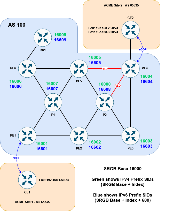
Here is the topology we will be working with:

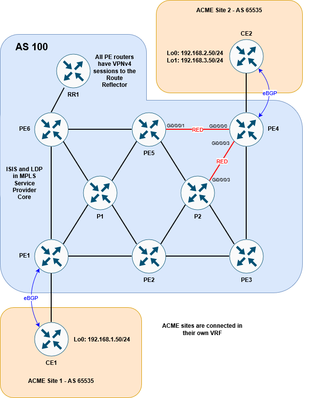
It’s a basic MPLS network, running ISIS + LDP in the core. VPNv4 routes are exchanged via the router reflector. CE1 and CE2 are customer devices connected via BGP to the Service Provider – placed inside VRF ACME.
I’ve built this lab in EVE-NG. If you have your own setup, you can download the lab and/or config files here to follow along:


The EVE-NG lab consists of:
11 x Cisco XRv 9k 7.9.2s and 2 x Cisco XE 17.03.02s
Login creds are user1/user123
The goal
As mentioned above, our goal here is to connect two SR policies together. The first policy will direct traffic from PE1 to PE5 using an explicit path. The second policy will direct traffic from PE5 to PE4 by dynamically avoiding red colored links.
Here it is in diagram form:

Whilst this is only a lab environment, this kind of traffic engineering could be used in larger environments to do tasks such as steering traffic towards DDoS scrubbers, avoiding maintenance links or crossing administrative boundaries.
If we were using MPLS RSVP to signal the separate paths, all the LSRs would need to reserve and maintain the required state. This would be done using RSVP Path or Resv message (more details here). Segment Routing can accomplish this much more efficiently.
We’ll begin by looking at the base state of the network, then walk through the steps to enable SR, before finally creating the policies.
The setup
Let’s start by checking out the ISIS and LDP config. Here is a sample from PE1:
RP/0/RP0/CPU0:PE1#sh run router isis
Fri Nov  7 20:20:35.436 UTC
router isis ISIS1
 is-type level-2-only
 net 49.0001.0100.0000.0001.00
 mpls ldp sync
 address-family ipv4 unicast
  metric-style wide
  advertise passive-only
  mpls ldp auto-config
 !
 address-family ipv6 unicast
  metric-style wide
  advertise passive-only
  single-topology
 !
 interface Loopback0
  passive
  address-family ipv4 unicast
  !
  address-family ipv6 unicast
  !
 !
 interface GigabitEthernet0/0/0/0
  point-to-point
  address-family ipv4 unicast
  !
  address-family ipv6 unicast
  !
 !
 interface GigabitEthernet0/0/0/2
  point-to-point
  address-family ipv4 unicast
  !
  address-family ipv6 unicast
  !
 !
 interface GigabitEthernet0/0/0/3
  point-to-point
  address-family ipv4 unicast
  !
  address-family ipv6 unicast
  !
 !
!

RP/0/RP0/CPU0:PE1#
PE1 has a VRF called ACME configured with a BGP session to the CE2:
RP/0/RP0/CPU0:PE1#sh run router bgp
Fri Nov  7 20:21:03.711 UTC
router bgp 100
 address-family vpnv4 unicast
 !
 address-family vpnv6 unicast
 !
 neighbor-group RR
  remote-as 100
  update-source Loopback0
  address-family vpnv4 unicast
  !
  address-family vpnv6 unicast
  !
 !
 neighbor 10.1.1.9
  use neighbor-group RR
 !
 vrf ACME
  address-family ipv4 unicast
  !
  address-family ipv6 unicast
  !
  neighbor 172.16.1.2
   remote-as 65535
   address-family ipv4 unicast
    route-policy ALLOW-ALL in
    route-policy ALLOW-ALL out
    as-override
   !
  !
  neighbor 2001:ce1::2
   remote-as 65535
   address-family ipv6 unicast
    route-policy ALLOW-ALL in
    route-policy ALLOW-ALL out
    as-override
   !
  !
 !
!

RP/0/RP0/CPU0:PE1# sh bgp vrf ACME neighbors 172.16.1.2 routes
Fri Nov  7 20:21:23.859 UTC
BGP VRF ACME, state: Active
BGP Route Distinguisher: 100:1
VRF ID: 0x60000001
BGP router identifier 10.1.1.1, local AS number 100
Non-stop routing is enabled
BGP table state: Active
Table ID: 0xe0000001   RD version: 10
BGP main routing table version 10
BGP NSR Initial initsync version 4 (Reached)
BGP NSR/ISSU Sync-Group versions 0/0

Status codes: s suppressed, d damped, h history, * valid, > best
              i - internal, r RIB-failure, S stale, N Nexthop-discard
Origin codes: i - IGP, e - EGP, ? - incomplete
   Network            Next Hop            Metric LocPrf Weight Path
Route Distinguisher: 100:1 (default for vrf ACME)
Route Distinguisher Version: 10
*> 192.168.1.0/24     172.16.1.2               0             0 65535 i

Processed 1 prefixes, 1 paths
RP/0/RP0/CPU0:PE1#
The same type of session is configured between PE4 and CE2. This is all fairly stock standard for a Service Provider environment. We can demonstrate the basic MPLS network by running a traceroute from CE1 to CE2 (sourcing with CE1 Loopback 0 to emulate a LAN).
(NB. For the sake of this lab, the label ranges for each if the LSRs have been set to 24×00 – 24×99, where x is the identifier for that router – PE1 has identifier 1 etc.)
CE1#traceroute 192.168.2.50 source lo0
Type escape sequence to abort.
Tracing the route to 192.168.2.50
VRF info: (vrf in name/id, vrf out name/id)
  1 172.16.1.1 3 msec 2 msec 2 msec
  2 10.10.16.6 [MPLS: Labels 24607/24407 Exp 0] 4 msec
    10.10.17.7 [MPLS: Labels 24707/24407 Exp 0] 4 msec 4 msec
  3 10.10.57.5 [MPLS: Labels 24507/24407 Exp 0] 3 msec
    10.10.56.5 [MPLS: Labels 24507/24407 Exp 0] 3 msec 3 msec
  4 10.10.45.4 [MPLS: Label 24407 Exp 0] 4 msec
    10.10.48.4 [MPLS: Label 24407 Exp 0] 3 msec
    10.10.45.4 [MPLS: Label 24407 Exp 0] 3 msec
  5 172.16.2.2 3 msec *  5 msec
CE1#
You can see the traffic is taking a standard ECMP path through the network. Now let’s look at getting SR working
Setting up SR
Enable Segment Routing
The first step is to enable SR and assign prefix SIDs (don’t forget to enable mpls traffic engineering router-id as well!).
We’ll set the SRGB base to be 16000 across all devices and give sequential IPv4 indexes to each router (PE1 will be SID index 1 etc.). The IPv6 indexes will be the same but +600.
RP/0/RP0/CPU0:PE1#conf t
Fri Nov  7 20:23:21.489 UTC
RP/0/RP0/CPU0:PE1(config)#router isis ISIS1
RP/0/RP0/CPU0:PE1(config-isis)# address-family ipv4 unicast
RP/0/RP0/CPU0:PE1(config-isis-af)#  segment-routing mpls sr-prefer
RP/0/RP0/CPU0:PE1(config-isis-af)#  router-id lo0
RP/0/RP0/CPU0:PE1(config-isis-af)# !
RP/0/RP0/CPU0:PE1(config-isis-af)# address-family ipv6 unicast
RP/0/RP0/CPU0:PE1(config-isis-af)#  segment-routing mpls sr-prefer
RP/0/RP0/CPU0:PE1(config-isis-af)#  router-id lo0
RP/0/RP0/CPU0:PE1(config-isis-af)# !
RP/0/RP0/CPU0:PE1(config-isis-af)# interface Loopback0
RP/0/RP0/CPU0:PE1(config-isis-if)#  address-family ipv4 unicast
RP/0/RP0/CPU0:PE1(config-isis-if-af)#   prefix-sid index 1
RP/0/RP0/CPU0:PE1(config-isis-if-af)#  !
RP/0/RP0/CPU0:PE1(config-isis-if-af)#  address-family ipv6 unicast
RP/0/RP0/CPU0:PE1(config-isis-if-af)#   prefix-sid index 601
RP/0/RP0/CPU0:PE1(config-isis-if-af)#  !
RP/0/RP0/CPU0:PE1(config-isis-if-af)# !
RP/0/RP0/CPU0:PE1(config-isis-if-af)#!
RP/0/RP0/CPU0:PE1(config-isis-if-af)#segment-routing
RP/0/RP0/CPU0:PE1(config-sr)# global-block 16000 23999
RP/0/RP0/CPU0:PE1(config-sr)#commit
Fri Nov  7 20:24:01.542 UTC
RP/0/RP0/CPU0:Nov  7 20:24:03.706 UTC: bgp[1094]: %ROUTING-BGP-2-SR_CFG_CHANGED : SRGB range config has been changed. BGP's labels have to be re-programmed as per new range, 'process restart bgp' needed
RP/0/RP0/CPU0:PE1(config-sr)#
RP/0/RP0/CPU0:PE1#
I’ve enabled the router ID using the router-id lo0 command here, which works under ipv4 and ipv6. An alternative is to use mpls traffic-eng router-id lo0. This might already be in place if you are migrating from traditional MPLS-TE, but it’s only applicable to the ipv4 address-family.
Once we repeat this for all the Service Provider routers, we can see that the MPLS forwarding table now prefers Segment Routing:
RP/0/RP0/CPU0:PE1#sh mpls forwarding
Fri Nov  7 20:29:20.862 UTC
Local  Outgoing    Prefix             Outgoing     Next Hop        Bytes
Label  Label       or ID              Interface                    Switched
------ ----------- ------------------ ------------ --------------- ------------
16001  Aggregate   SR Pfx (idx 1)     default                      0
16002  Pop         SR Pfx (idx 2)     Gi0/0/0/3    10.10.12.2      0
16003  16003       SR Pfx (idx 3)     Gi0/0/0/3    10.10.12.2      0
16004  16004       SR Pfx (idx 4)     Gi0/0/0/0    10.10.16.6      0
       16004       SR Pfx (idx 4)     Gi0/0/0/3    10.10.12.2      0
       16004       SR Pfx (idx 4)     Gi0/0/0/2    10.10.17.7      0
16005  16005       SR Pfx (idx 5)     Gi0/0/0/0    10.10.16.6      0
       16005       SR Pfx (idx 5)     Gi0/0/0/3    10.10.12.2      0
       16005       SR Pfx (idx 5)     Gi0/0/0/2    10.10.17.7      0
16006  Pop         SR Pfx (idx 6)     Gi0/0/0/0    10.10.16.6      0
16007  Pop         SR Pfx (idx 7)     Gi0/0/0/2    10.10.17.7      0
16008  16008       SR Pfx (idx 8)     Gi0/0/0/3    10.10.12.2      0
16009  16009       SR Pfx (idx 9)     Gi0/0/0/0    10.10.16.6      0
16601  Aggregate   SR Pfx (idx 601)   default                      0
16602  Pop         SR Pfx (idx 602)   Gi0/0/0/3    fe80::5200:ff:fe05:6   \
                                                                   0
16603  16603       SR Pfx (idx 603)   Gi0/0/0/3    fe80::5200:ff:fe05:6   \
                                                                   0
16604  16604       SR Pfx (idx 604)   Gi0/0/0/0    fe80::5200:ff:fe02:4   \
                                                                   0
       16604       SR Pfx (idx 604)   Gi0/0/0/3    fe80::5200:ff:fe05:6   \
                                                                   0
       16604       SR Pfx (idx 604)   Gi0/0/0/2    fe80::5200:ff:fe04:5   \
                                                                   0
16605  16605       SR Pfx (idx 605)   Gi0/0/0/0    fe80::5200:ff:fe02:4   \
                                                                   0
       16605       SR Pfx (idx 605)   Gi0/0/0/3    fe80::5200:ff:fe05:6   \
                                                                   0
       16605       SR Pfx (idx 605)   Gi0/0/0/2    fe80::5200:ff:fe04:5   \
                                                                   0
16606  Pop         SR Pfx (idx 606)   Gi0/0/0/0    fe80::5200:ff:fe02:4   \
                                                                   0
16607  Pop         SR Pfx (idx 607)   Gi0/0/0/2    fe80::5200:ff:fe04:5   \
                                                                   0
16608  16608       SR Pfx (idx 608)   Gi0/0/0/3    fe80::5200:ff:fe05:6   \
                                                                   0
16609  16609       SR Pfx (idx 609)   Gi0/0/0/0    fe80::5200:ff:fe02:4   \
                                                                   59
24100  24600       10.1.1.9/32        Gi0/0/0/0    10.10.16.6      0
24101  Pop         10.1.1.6/32        Gi0/0/0/0    10.10.16.6      196
24102  24601       10.1.1.5/32        Gi0/0/0/0    10.10.16.6      0
       24204       10.1.1.5/32        Gi0/0/0/3    10.10.12.2      0
       24703       10.1.1.5/32        Gi0/0/0/2    10.10.17.7      0
24103  Pop         10.1.1.7/32        Gi0/0/0/2    10.10.17.7      98
24104  24201       10.1.1.8/32        Gi0/0/0/3    10.10.12.2      0
24105  24206       10.1.1.3/32        Gi0/0/0/3    10.10.12.2      0
24106  Unlabelled  192.168.1.0/24[V]  Gi0/0/0/1    172.16.1.2      0
24107  Unlabelled  2001:ac73:1::/64[V]   \
                                      Gi0/0/0/1    fe80::5200:ff:fe06:0   \
                                                                   0
24108  Pop         10.1.1.2/32        Gi0/0/0/3    10.10.12.2      334
24109  24607       10.1.1.4/32        Gi0/0/0/0    10.10.16.6      0
       24205       10.1.1.4/32        Gi0/0/0/3    10.10.12.2      0
       24707       10.1.1.4/32        Gi0/0/0/2    10.10.17.7      0
24110  Pop         SR Adj (idx 1)     Gi0/0/0/3    10.10.12.2      0
24111  Pop         SR Adj (idx 3)     Gi0/0/0/3    10.10.12.2      0
24112  Pop         SR Adj (idx 1)     Gi0/0/0/0    10.10.16.6      0
24113  Pop         SR Adj (idx 3)     Gi0/0/0/0    10.10.16.6      0
24114  Pop         SR Adj (idx 1)     Gi0/0/0/2    10.10.17.7      0
24115  Pop         SR Adj (idx 3)     Gi0/0/0/2    10.10.17.7      0
24116  Pop         SR Adj (idx 1)     Gi0/0/0/3    fe80::5200:ff:fe05:6   \
                                                                   0
24117  Pop         SR Adj (idx 3)     Gi0/0/0/3    fe80::5200:ff:fe05:6   \
                                                                   0
24118  Pop         SR Adj (idx 1)     Gi0/0/0/0    fe80::5200:ff:fe02:4   \
                                                                   0
24119  Pop         SR Adj (idx 3)     Gi0/0/0/0    fe80::5200:ff:fe02:4   \
                                                                   0
24120  Pop         SR Adj (idx 1)     Gi0/0/0/2    fe80::5200:ff:fe04:5   \
                                                                   0
24121  Pop         SR Adj (idx 3)     Gi0/0/0/2    fe80::5200:ff:fe04:5   \
                                                                   0
RP/0/RP0/CPU0:PE1#
And indeed, if we repeat our traceroute we can see that SR labels are now used:
CE1#traceroute 192.168.2.50 source lo0
Type escape sequence to abort.
Tracing the route to 192.168.2.50
VRF info: (vrf in name/id, vrf out name/id)
  1 172.16.1.1 3 msec 1 msec 2 msec
  2 10.10.16.6 [MPLS: Labels 16004/24407 Exp 0] 5 msec
    10.10.17.7 [MPLS: Labels 16004/24407 Exp 0] 4 msec
    10.10.16.6 [MPLS: Labels 16004/24407 Exp 0] 4 msec
  3 10.10.56.5 [MPLS: Labels 16004/24407 Exp 0] 3 msec 3 msec
    10.10.57.5 [MPLS: Labels 16004/24407 Exp 0] 3 msec
  4 10.10.45.4 [MPLS: Label 24407 Exp 0] 4 msec
    10.10.48.4 [MPLS: Label 24407 Exp 0] 4 msec
    10.10.45.4 [MPLS: Label 24407 Exp 0] 3 msec
  5 172.16.2.2 3 msec *  4 msec
CE1#
ECMP is still in effect, but since the transport label stays as 16004 the whole way, we’d need to look at the IP addresses to determine the exact path.
Populate SRTE Database
From here we need to populate the SRTE database so that any dynamic policies (in our case the one that avoids RED links) can calculate their best path. This is done using the distribute link-state command under ISIS:
RP/0/RP0/CPU0:PE1#conf t
Fri Nov  7 20:30:46.177 UTC
RP/0/RP0/CPU0:PE1(config)#router isis ISIS1
RP/0/RP0/CPU0:PE1(config-isis)#distribute link-state
RP/0/RP0/CPU0:PE1(config-isis)#commit
Fri Nov  7 20:31:05.594 UTC
RP/0/RP0/CPU0:PE1(config-isis)#
RP/0/RP0/CPU0:PE1#
Once this is done across all the devices, we can see the topology by running the following command:
RP/0/RP0/CPU0:PE2#show segment-routing traffic-eng topology
Fri Nov  7 20:32:16.003 UTC

Topology database:
------------------
Node 11
  Router ID: 10.1.1.1

  ISIS-L2 0100.0000.0001
    Hostname: PE1
    TE router ID: 10.1.1.1
    IPv6 router ID: 2001:1ab::1
    ISIS area ID: 49.0001
    SRGBs: 16000 - 24000
    SRLBs: 15000 - 16000

    Prefixes:
      10.1.1.1/32
        Regular SID index: 1
      2001:1ab::1/128
        Regular SID index: 601

    Links:
      Local: 10.10.12.1 Remote: 10.10.12.2
        Remote node: ISIS-L2 0100.0000.0002
          Hostname: PE2
          TE router ID: 10.1.1.2
          IPv6 router ID: 2001:1ab::2
          ISIS area ID: 49.0001
        Metrics: IGP 10
        Bandwidth: Total 125000000 Bps, Reservable 0 Bps
        Adj-SIDs: 24111 (unprotected), 24117 (unprotected)

      Local: 10.10.16.1 Remote: 10.10.16.6
        Remote node: ISIS-L2 0100.0000.0006
          Hostname: PE6
          TE router ID: 10.1.1.6
          IPv6 router ID: 2001:1ab::6
          ISIS area ID: 49.0001
        Metrics: IGP 10
        Bandwidth: Total 125000000 Bps, Reservable 0 Bps
        Adj-SIDs: 24113 (unprotected), 24119 (unprotected)

      Local: 10.10.17.1 Remote: 10.10.17.7
        Remote node: ISIS-L2 0100.0000.0007
          Hostname: P1
          TE router ID: 10.1.1.7
          IPv6 router ID: 2001:1ab::7
          ISIS area ID: 49.0001
        Metrics: IGP 10
        Bandwidth: Total 125000000 Bps, Reservable 0 Bps
        Adj-SIDs: 24115 (unprotected), 24121 (unprotected)

<snip>

Node 19
  Router ID: 10.1.1.9

  ISIS-L2 0100.0000.0009
    Hostname: RR1
    TE router ID: 10.1.1.9
    IPv6 router ID: 2001:1ab::9
    ISIS area ID: 49.0001
    SRGBs: 16000 - 24000
    SRLBs: 15000 - 16000

    Prefixes:
      10.1.1.9/32
        Regular SID index: 9
      2001:1ab::9/128
        Regular SID index: 609

    Links:
      Local: 10.10.69.9 Remote: 10.10.69.6
        Remote node: ISIS-L2 0100.0000.0006
          Hostname: PE6
          TE router ID: 10.1.1.6
          IPv6 router ID: 2001:1ab::6
          ISIS area ID: 49.0001
        Metrics: IGP 10
        Bandwidth: Total 125000000 Bps, Reservable 0 Bps
        Adj-SIDs: 24909 (unprotected), 24911 (unprotected)

RP/0/RP0/CPU0:PE2#
RP/0/RP0/CPU0:PE2#show segment-routing traffic-eng topology | inc "Node|Local|Bind"
Fri Nov  7 20:33:42.222 UTC
Node 11
    Hostname: PE1
      Local: 10.10.12.1 Remote: 10.10.12.2
          Hostname: PE2
      Local: 10.10.16.1 Remote: 10.10.16.6
          Hostname: PE6
      Local: 10.10.17.1 Remote: 10.10.17.7
          Hostname: P1
Node 12
    Hostname: PE2
      Local: 10.10.12.2 Remote: 10.10.12.1
          Hostname: PE1
      Local: 10.10.23.2 Remote: 10.10.23.3
          Hostname: PE3
      Local: 10.10.25.2 Remote: 10.10.25.5
          Hostname: PE5
      Local: 10.10.27.2 Remote: 10.10.27.7
          Hostname: P1
      Local: 10.10.28.2 Remote: 10.10.28.8
          Hostname: P2
Node 13
    Hostname: PE3
      Local: 10.10.23.3 Remote: 10.10.23.2
          Hostname: PE2
      Local: 10.10.34.3 Remote: 10.10.34.4
          Hostname: PE4
      Local: 10.10.38.3 Remote: 10.10.38.8
          Hostname: P2
Node 14
    Hostname: PE5
      Local: 10.10.25.5 Remote: 10.10.25.2
          Hostname: PE2
      Local: 10.10.45.5 Remote: 10.10.45.4
          Hostname: PE4
      Local: 10.10.56.5 Remote: 10.10.56.6
          Hostname: PE6
      Local: 10.10.57.5 Remote: 10.10.57.7
          Hostname: P1
      Local: 10.10.58.5 Remote: 10.10.58.8
          Hostname: P2
Node 15
    Hostname: P1
      Local: 10.10.17.7 Remote: 10.10.17.1
          Hostname: PE1
      Local: 10.10.27.7 Remote: 10.10.27.2
          Hostname: PE2
      Local: 10.10.57.7 Remote: 10.10.57.5
          Hostname: PE5
      Local: 10.10.67.7 Remote: 10.10.67.6
          Hostname: PE6
Node 16
    Hostname: PE4
      Local: 10.10.34.4 Remote: 10.10.34.3
          Hostname: PE3
      Local: 10.10.45.4 Remote: 10.10.45.5
          Hostname: PE5
      Local: 10.10.48.4 Remote: 10.10.48.8
          Hostname: P2
Node 17
    Hostname: PE6
      Local: 10.10.16.6 Remote: 10.10.16.1
          Hostname: PE1
      Local: 10.10.56.6 Remote: 10.10.56.5
          Hostname: PE5
      Local: 10.10.67.6 Remote: 10.10.67.7
          Hostname: P1
      Local: 10.10.69.6 Remote: 10.10.69.9
          Hostname: RR1
Node 18
    Hostname: P2
      Local: 10.10.28.8 Remote: 10.10.28.2
          Hostname: PE2
      Local: 10.10.38.8 Remote: 10.10.38.3
          Hostname: PE3
      Local: 10.10.48.8 Remote: 10.10.48.4
          Hostname: PE4
      Local: 10.10.58.8 Remote: 10.10.58.5
          Hostname: PE5
Node 19
    Hostname: RR1
      Local: 10.10.69.9 Remote: 10.10.69.6
          Hostname: PE6
RP/0/RP0/CPU0:PE2#
All devices within the same domain should show the same output. We are now ready to start setting up the policies.
Configure explicit SR Policy
The first thing to do is set up an explicit segment list that details the path we want the traffic to follow. In our case the path looks like this:

Here is the CLI:
RP/0/RP0/CPU0:PE1#conf t
Fri Nov  7 20:34:54.088 UTC
RP/0/RP0/CPU0:PE1(config)#segment-routing traffic-eng
RP/0/RP0/CPU0:PE1(config-sr-te)#segment-list name LIST-TO-PE5
RP/0/RP0/CPU0:PE1(config-sr-te-sl)#index 10 mpls label 16006
RP/0/RP0/CPU0:PE1(config-sr-te-sl)#index 20 mpls label 16007
RP/0/RP0/CPU0:PE1(config-sr-te-sl)#index 30 mpls label 16005
RP/0/RP0/CPU0:PE1(config-sr-te-sl)#commit
Fri Nov  7 20:34:59.279 UTC
RP/0/RP0/CPU0:PE1(config-sr-te-sl)#
RP/0/RP0/CPU0:PE1#
With this done, we can create an SR policy to reference the explicit path:
RP/0/RP0/CPU0:PE1#conf t
Fri Nov  7 20:36:17.083 UTC
RP/0/RP0/CPU0:PE1(config)#segment-routing traffic-eng
RP/0/RP0/CPU0:PE1(config-sr-te)#policy TO-PE5
RP/0/RP0/CPU0:PE1(config-sr-te-policy)#color 10 end-point ipv4 10.1.1.5
RP/0/RP0/CPU0:PE1(config-sr-te-policy)#candidate-paths preference 100
RP/0/RP0/CPU0:PE1(config-sr-te-policy-path-pref)#explicit segment-list LIST-TO-PE5
RP/0/RP0/CPU0:PE1(config-sr-te-pp-info)#commit
Fri Nov  7 20:37:23.704 UTC
RP/0/RP0/CPU0:PE1(config-sr-te-pp-info)#
RP/0/RP0/CPU0:PE1#
So far so good. Let’s verify that it has come up okay:
RP/0/RP0/CPU0:PE1#show segment-routing traffic-eng policy color 10
Fri Nov  7 20:38:39.694 UTC

SR-TE policy database
---------------------

Color: 10, End-point: 10.1.1.5
  Name: srte_c_10_ep_10.1.1.5
  Status:
    Admin: up  Operational: up for 00:01:14 (since Nov  7 20:37:24.854)
  Candidate-paths:
    Preference: 100 (configuration) (active)
      Name: TO-PE5
      Requested BSID: dynamic
      Constraints:
        Protection Type: protected-preferred
        Maximum SID Depth: 10
      Explicit: segment-list LIST-TO-PE5 (valid)
        Weight: 1, Metric Type: TE
          SID[0]: 16006 [Prefix-SID, 10.1.1.6]
          SID[1]: 16007
          SID[2]: 16005
  Attributes:
    Binding SID: 24123
    Forward Class: Not Configured
    Steering labeled-services disabled: no
    Steering BGP disabled: no
    IPv6 caps enable: yes
    Invalidation drop enabled: no
    Max Install Standby Candidate Paths: 0

RP/0/RP0/CPU0:PE1#
We can see from the policy that it is up, but how do we steer traffic into it?
This is done by attaching a color community to the BGP router that matches the color of the policy. In our case, we’ll tag 192.168.2.0/24 inbound from CE2 with color 10

RP/0/RP0/CPU0:PE4#conf t
Fri Nov  7 20:41:21.957 UTC
RP/0/RP0/CPU0:PE4(config)#extcommunity-set opaque COLOR-10
RP/0/RP0/CPU0:PE4(config-ext)#10
RP/0/RP0/CPU0:PE4(config-ext)#end-set
RP/0/RP0/CPU0:PE4(config)#route-policy FROM-CE2
RP/0/RP0/CPU0:PE4(config-rpl)#if destination in (192.168.2.0/24) then
RP/0/RP0/CPU0:PE4(config-rpl-if)#set extcommunity color COLOR-10
RP/0/RP0/CPU0:PE4(config-rpl-if)#endif
RP/0/RP0/CPU0:PE4(config-rpl)#pass
RP/0/RP0/CPU0:PE4(config-rpl)#end-policy
RP/0/RP0/CPU0:PE4(config)#router bgp 100
RP/0/RP0/CPU0:PE4(config-bgp)#vrf ACME
RP/0/RP0/CPU0:PE4(config-bgp-vrf)#neighbor 172.16.2.2
RP/0/RP0/CPU0:PE4(config-bgp-vrf-nbr)#address-family ipv4 unicast
RP/0/RP0/CPU0:PE4(config-bgp-vrf-nbr-af)#route-policy FROM-CE2 in
RP/0/RP0/CPU0:PE4(config-bgp-vrf-nbr-af)#
Before we commit, here is what the prefix currently looks like in the BGP table:
RP/0/RP0/CPU0:PE4(config-bgp-vrf-nbr-af)#do show bgp vrf ACME 192.168.2.0
Fri Nov  7 20:41:50.516 UTC
BGP routing table entry for 192.168.2.0/24, Route Distinguisher: 100:1
Versions:
  Process           bRIB/RIB  SendTblVer
  Speaker                  14           14
    Local Label: 24407
Last Modified: Nov  7 20:41:20.501 for 00:00:30
Paths: (1 available, best #1)
  Advertised to PE peers (in unique update groups):
    10.1.1.9
  Path #1: Received by speaker 0
  Advertised to PE peers (in unique update groups):
    10.1.1.9
  65535
    172.16.2.2 from 172.16.2.2 (192.168.3.50)
      Origin IGP, metric 0, localpref 100, valid, external, best, group-best, import-candidate
      Received Path ID 0, Local Path ID 1, version 14
      Extended community: RT:100:1
      Origin-AS validity: (disabled)
RP/0/RP0/CPU0:PE4(config-bgp-vrf-nbr-af)#
The additon of the color can be seen once we commit:
RP/0/RP0/CPU0:PE4(config-bgp-vrf-nbr-af)#commit
Fri Nov  7 20:42:10.086 UTC
RP/0/RP0/CPU0:PE4(config-bgp-vrf-nbr-af)#
RP/0/RP0/CPU0:PE4#show bgp vrf ACME 192.168.2.0
Fri Nov  7 20:42:19.644 UTC
BGP routing table entry for 192.168.2.0/24, Route Distinguisher: 100:1
Versions:
  Process           bRIB/RIB  SendTblVer
  Speaker                  16           16
    Local Label: 24407
Last Modified: Nov  7 20:42:12.501 for 00:00:07
Paths: (1 available, best #1)
  Advertised to PE peers (in unique update groups):
    10.1.1.9
  Path #1: Received by speaker 0
  Advertised to PE peers (in unique update groups):
    10.1.1.9
  65535
    172.16.2.2 from 172.16.2.2 (192.168.3.50)
      Origin IGP, metric 0, localpref 100, valid, external, best, group-best, import-candidate
      Received Path ID 0, Local Path ID 1, version 16
      Extended community: Color:10 RT:100:1
      Origin-AS validity: (disabled)
RP/0/RP0/CPU0:PE4#
Note that this has only been applied to 192.168.2.0/24, not 192.168.3.0/24:
RP/0/RP0/CPU0:PE4#show bgp vrf ACME 192.168.3.0
Fri Nov  7 20:42:53.104 UTC
BGP routing table entry for 192.168.3.0/24, Route Distinguisher: 100:1
Versions:
  Process           bRIB/RIB  SendTblVer
  Speaker                  15           15
    Local Label: 24409
Last Modified: Nov  7 20:41:20.501 for 00:01:32
Paths: (1 available, best #1)
  Advertised to PE peers (in unique update groups):
    10.1.1.9
  Path #1: Received by speaker 0
  Advertised to PE peers (in unique update groups):
    10.1.1.9
  65535
    172.16.2.2 from 172.16.2.2 (192.168.3.50)
      Origin IGP, metric 0, localpref 100, valid, external, best, group-best, import-candidate
      Received Path ID 0, Local Path ID 1, version 15
      Extended community: RT:100:1
      Origin-AS validity: (disabled)
RP/0/RP0/CPU0:PE4#
PE1 sees the color as well:
RP/0/RP0/CPU0:PE1#sh bgp vrf ACME 192.168.2.0/24
Fri Nov  7 20:43:32.410 UTC
BGP routing table entry for 192.168.2.0/24, Route Distinguisher: 100:1
Versions:
  Process           bRIB/RIB  SendTblVer
  Speaker                  18           18
Last Modified: Nov  7 20:42:12.284 for 00:01:20
Paths: (1 available, best #1)
  Advertised to CE peers (in unique update groups):
    172.16.1.2
  Path #1: Received by speaker 0
  Advertised to CE peers (in unique update groups):
    172.16.1.2
  65535
    10.1.1.4 (metric 30) from 10.1.1.9 (10.1.1.4)
      Received Label 24407
      Origin IGP, metric 0, localpref 100, valid, internal, best, group-best, import-candidate, imported
      Received Path ID 0, Local Path ID 1, version 18
      Extended community: Color:10 RT:100:1
      Originator: 10.1.1.4, Cluster list: 10.1.1.9
      Source AFI: VPNv4 Unicast, Source VRF: ACME, Source Route Distinguisher: 100:1
RP/0/RP0/CPU0:PE1#
The idea here is for traffic to 192.168.20/24 to be directed into our color 10 tunnel. If this is working, we should see the CEF table on the ACME VRF recurving to the Binding SID for our SR Policy (if you look above, the Binding SID is 24123)…
RP/0/RP0/CPU0:PE1#show cef vrf ACME 192.168.2.0
Fri Nov  7 20:44:08.498 UTC
192.168.2.0/24, version 17, internal 0x5000001 0x30 (ptr 0xe9d5288) [1], 0x600 (0xd6f8dd8), 0xa08 (0xf549510)
 Updated Nov  7 20:42:11.812
 Prefix Len 24, traffic index 0, precedence n/a, priority 3
  gateway array (0xd5524d8) reference count 2, flags 0x38, source rib (7), 0 backups
                [3 type 1 flags 0x8441 (0xf583358) ext 0x0 (0x0)]
  LW-LDI[type=1, refc=1, ptr=0xd6f8dd8, sh-ldi=0xf583358]
  gateway array update type-time 1 Nov  7 20:41:19.728
 LDI Update time Nov  7 20:41:19.729
 LW-LDI-TS Nov  7 20:41:19.729
   via 10.1.1.4/32, 5 dependencies, recursive [flags 0x6000]
    path-idx 0 NHID 0x0 [0xd8bf740 0x0]
    recursion-via-/32
    next hop VRF - 'default', table - 0xe0000000
    next hop 10.1.1.4/32 via 16004/0/21
     next hop 10.10.16.6/32 Gi0/0/0/0    labels imposed {16004 24407}
     next hop 10.10.12.2/32 Gi0/0/0/3    labels imposed {16004 24407}
     next hop 10.10.17.7/32 Gi0/0/0/2    labels imposed {16004 24407}

    Load distribution: 0 (refcount 3)

    Hash  OK  Interface                 Address
    0     Y   recursive                 16004/0
RP/0/RP0/CPU0:PE1#
But here, it looks like it is still just imposing 16004 (the SID for R4) and then 24407 (the VPNv4 label for 192.168.2.0/24). It’s then ECMP’ing it out of Gi0/0/0/0, Gi0/0/0/3 and Gi0/0/0/2.
So what gives? Why is it not using our SR Policy?
Well, we have to remember that the allocation of a prefix to a policy is based on the combination of the end-point and the color. Looking at the BGP route, the color is correct, but the end point (or next-hop in BGP talk) is still 10.1.1.4 – PE4. Our policy is defined as having an end-point of 10.1.1.5!
So let’s fix that:
RP/0/RP0/CPU0:PE1#conf t
Fri Nov  7 20:45:04.898 UTC
RP/0/RP0/CPU0:PE1(config)#segment-routing traffic-eng
RP/0/RP0/CPU0:PE1(config-sr-te)#policy TO-PE5
RP/0/RP0/CPU0:PE1(config-sr-te-policy)#color 10 end-point ipv4 10.1.1.4
RP/0/RP0/CPU0:PE1(config-sr-te-policy)#commit
Fri Nov  7 20:45:31.664 UTC
RP/0/RP0/CPU0:PE1(config-sr-te-policy)#
RP/0/RP0/CPU0:PE1#
Now we see that it is correctly steering down the SR policy:
RP/0/RP0/CPU0:PE1#sh segment-routing traffic-eng policy color 10 | inc "Operation|Bind"
Fri Nov  7 20:46:53.444 UTC
    Admin: up  Operational: up for 00:01:21 (since Nov  7 20:45:31.897)
    Binding SID: 24125
RP/0/RP0/CPU0:PE1#show cef vrf ACME 192.168.2.0
Fri Nov  7 20:47:05.492 UTC
192.168.2.0/24, version 21, internal 0x5000001 0x30 (ptr 0xe9d5288) [1], 0x600 (0xd6f8dd8), 0xa08 (0xf54a068)
 Updated Nov  7 20:45:31.910
 Prefix Len 24, traffic index 0, precedence n/a, priority 3
  gateway array (0xd553440) reference count 1, flags 0x38, source rib (7), 0 backups
                [2 type 1 flags 0x8441 (0xf584328) ext 0x0 (0x0)]
  LW-LDI[type=1, refc=1, ptr=0xd6f8dd8, sh-ldi=0xf584328]
  gateway array update type-time 1 Nov  7 20:45:31.910
 LDI Update time Nov  7 20:45:31.910
 LW-LDI-TS Nov  7 20:45:31.910
   via local-label 24125, 3 dependencies, recursive [flags 0x6000]
    path-idx 0 NHID 0x0 [0xd8bb388 0x0]
    recursion-via-label
    next hop VRF - 'default', table - 0xe0000000
    next hop via 24125/0/21
     next hop srte_c_10_ep labels imposed {ImplNull 24407}

    Load distribution: 0 (refcount 2)

    Hash  OK  Interface                 Address
    0     Y   recursive                 24125/0
RP/0/RP0/CPU0:PE1#
The Binding SID has changed to 24125 since we refreshed the endpoint, but CEF is looking good.
However, whilst this is steering the traffic into the policy, it still won’t get us all the way. If trace from CE1 we can see that we just get stars:
CE1#traceroute 192.168.2.50 source lo0
Type escape sequence to abort.
Tracing the route to 192.168.2.50
VRF info: (vrf in name/id, vrf out name/id)
  1 172.16.1.1 47 msec 1 msec 2 msec
  2  *  *  *
  3  *  *  *
  4  *  *  *
  5  *  *  *
  6  *  *  *
  7  *
CE1#
The reason for this is fairly simple. This is the stack we are putting on the packet to CE2:
16006 (PE6 Prefix SID)
16007 (P1 Prefix SID)
16005 (PE5 Prefix SID)
24407 (VPN label)
As each segment is completed, the top label is popped. We can very quickly see that when the packet reaches PE5 the VPN label is exposed. But PE5 has no idea what to do with it! This VPN label was allocated by PE4 not PE5!
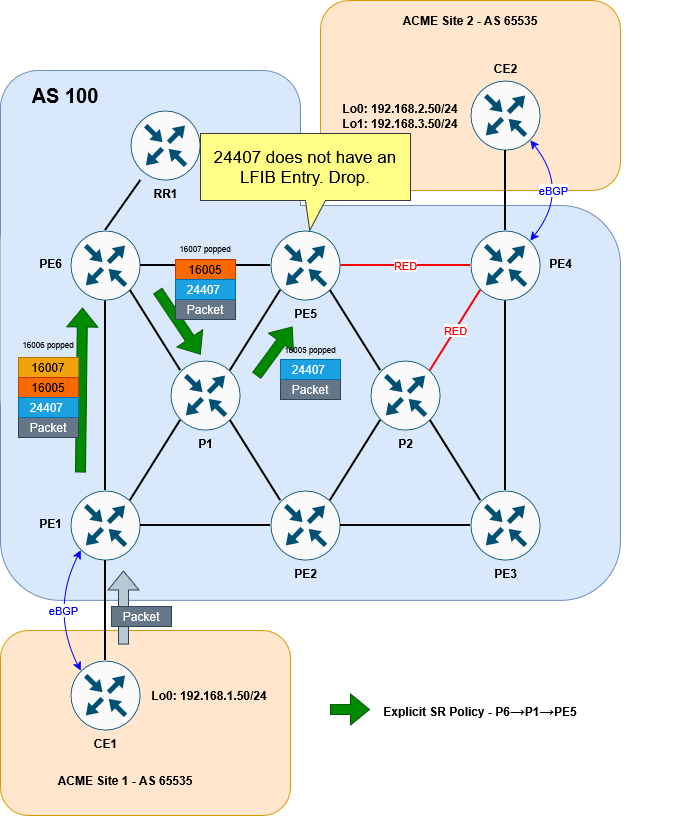
For our solution, this is okay at this point in the setup. Remember we will be wanting to push this traffic into a second policy that avoids all RED links and does end up at PE4.
For now, and just for the sake of getting our traceroute working, let’s add the PE4 label to the bottom of our explicit stack, so that PE5 can forward traffic on to PE4. We’ll remove this later:
RP/0/RP0/CPU0:PE1#conf t
Fri Nov  7 20:49:52.903 UTC
RP/0/RP0/CPU0:PE1(config)#segment-routing
RP/0/RP0/CPU0:PE1(config-sr)#traffic-eng
RP/0/RP0/CPU0:PE1(config-sr-te)#segment-list LIST-TO-PE5
RP/0/RP0/CPU0:PE1(config-sr-te-sl)#index 40 mpls label 16004
RP/0/RP0/CPU0:PE1(config-sr-te-sl)#commit
Fri Nov  7 20:50:03.914 UTC
RP/0/RP0/CPU0:PE1(config-sr-te-sl)#
RP/0/RP0/CPU0:PE1#
Now a traceroute works correctly:
CE1#traceroute 192.168.2.50 source lo0
Type escape sequence to abort.
Tracing the route to 192.168.2.50
VRF info: (vrf in name/id, vrf out name/id)
  1 172.16.1.1 3 msec 2 msec 2 msec
  2 10.10.16.6 [MPLS: Labels 16007/16005/16004/24407 Exp 0] 5 msec 3 msec 4 msec
  3 10.10.67.7 [MPLS: Labels 16005/16004/24407 Exp 0] 4 msec 3 msec 3 msec
  4 10.10.57.5 [MPLS: Labels 16004/24407 Exp 0] 7 msec 3 msec 3 msec
  5 10.10.45.4 [MPLS: Label 24407 Exp 0] 3 msec 3 msec 3 msec
  6 172.16.2.2 3 msec *  5 msec
CE1#
For the explicit path to PE5 to work, we need to make sure that a label that PE5 is going to understand is exposed. To get that, we need to configure the second policy from PE4…
Configure dynamic SR Policy
This policy isn’t going to be explicitly defined. Rather, we’re going to define the conditions of the policy (namely to avoid red links) and let the head end router figure it out. The first step in creating a dynamic policy that avoids red links is to, well, configure some RED links!
As a reminder, these are the links we want to color red:
Before going any further, let’s get some clarity on the term color and the different ways it is used within the context of this lab.
Color
This scenario uses the term color to refer to multiple different things and it can get confusing if you don’t know what you’re looking at. The two ways we’re concerned with color are as follows:
Policy Coloring
The first, is the color that we have already seen when defining an SR policy. This is an identifier for the policy. If a prefix is tagged with that color (in the case of BGP, it will be an attribute) and its next-hop matches the policy endpoint, traffic to that prefix will be steered into the policy. This is exactly how we’ve steered traffic into our explicit tunnel at PE1.
Link Coloring
The second way in which color is used is with regards to link coloring. Coloring a connection between two devices works by using something called link affinities (also called Admin group from the MPLS TE RSVP days). When we entered the distribute-link state command above, ISIS started to advertise Segment Routing details in its TLVs. This includes details about the links themselves – like metric, delay and link affinities. The link affinity is basically a string made up of ones and zeros that we can set and use how we wish. In this case, we’re using the affinity to “color” a link. I put the word “color” in air quotes, because from a CLI perspective, the word color isn’t actually referenced. We engineers use the term color because it’s easy to visualise a link that way.
This section looks at the latter of the two color definitions. Within the CLI the link-affinity is referenced as an integer number. For our scenario, let’s make 7 represent RED. Here’s how it would look:
RP/0/RP0/CPU0:PE4#conf t
Fri Nov  7 20:52:55.870 UTC
RP/0/RP0/CPU0:PE4(config)#segment-routing traffic-eng
RP/0/RP0/CPU0:PE4(config-sr-te)#affinity-map name RED bit-position 7
RP/0/RP0/CPU0:PE4(config-sr-te)#interface GigabitEthernet0/0/0/0
RP/0/RP0/CPU0:PE4(config-sr-if)#affinity
RP/0/RP0/CPU0:PE4(config-sr-if-affinity)#name RED
RP/0/RP0/CPU0:PE4(config-sr-if-affinity)#interface GigabitEthernet0/0/0/3
RP/0/RP0/CPU0:PE4(config-sr-if)#affinity
RP/0/RP0/CPU0:PE4(config-sr-if-affinity)#name RED
RP/0/RP0/CPU0:PE4(config-sr-if-affinity)#commit
Fri Nov  7 20:53:04.345 UTC
RP/0/RP0/CPU0:PE4(config-sr-if-affinity)#
RP/0/RP0/CPU0:PE4#
NB. As a side note, if you are configuring colors for different Flex-Algos, that config would go under the IGP (ISIS) and not under segment-routing. I won’t detail this here, but the principle of link coloring, with or without Flex-Algo, is the same.
Now that we’ve colored the link we can verify it:
RP/0/RP0/CPU0:PE4#show segment-routing traffic-eng topology | inc "Host|Link|Admin"
Fri Nov  7 20:54:14.682 UTC
<snip>
    Hostname: PE4
    Links:
          Hostname: PE3
          Hostname: PE5
        Admin groups: 0x00000080 0x00000000 0x00000000 0x00000000
          Hostname: P2
        Admin groups: 0x00000080 0x00000000 0x00000000 0x00000000
<snip>
RP/0/RP0/CPU0:PE4#
The output is a little messy, so I’ve piped the command and omitted the full result, but you can clearly see that the affinity bits (Admin groups) have been set for PE4’s links to PE5 and P2.
The next step would be to configure the policy on PE5 to avoid RED links. This looks similar to the explicit policy we used before but it instead uses the (surprise, surprise) dynamic keyword. We’ll give the policy a the color number of 20 (in the SR policy sense, not the link color sense), just to differentiate it from the PE1 – although colors will be locally significant:
RP/0/RP0/CPU0:PE5#conf t
Fri Nov  7 20:57:40.548 UTC
RP/0/RP0/CPU0:PE5(config)#segment-routing traffic-eng
RP/0/RP0/CPU0:PE5(config-sr-te)#policy AVOID-RED
RP/0/RP0/CPU0:PE5(config-sr-te-policy)#color 20 end-point ipv4 10.1.1.4
RP/0/RP0/CPU0:PE5(config-sr-te-policy)#candidate-paths preference 100
RP/0/RP0/CPU0:PE5(config-sr-te-policy-path-pref)#dynamic
RP/0/RP0/CPU0:PE5(config-sr-te-pp-info)#exit
RP/0/RP0/CPU0:PE5(config-sr-te-policy-path-pref)#constraints
RP/0/RP0/CPU0:PE5(config-sr-te-path-pref-const)#affinity
RP/0/RP0/CPU0:PE5(config-sr-te-path-pref-const-aff)#exclude-any name RED
RP/0/RP0/CPU0:PE5(config-sr-te-path-pref-const-aff)#commit
Fri Nov  7 20:57:45.688 UTC
RP/0/RP0/CPU0:PE5(config-sr-te-path-pref-const-aff)#
RP/0/RP0/CPU0:PE5#
Great. Now if we check the policy, we can see that it is up:
RP/0/RP0/CPU0:PE5#sh segment-routing traffic-eng policy color 20
Fri Nov  7 21:15:12.580 UTC

SR-TE policy database
---------------------

Color: 20, End-point: 10.1.1.4
  Name: srte_c_20_ep_10.1.1.4
  Status:
    Admin: up  Operational: up for 00:06:00 (since Nov  7 21:09:12.560)
  Candidate-paths:
    Preference: 100 (configuration) (active)
      Name: AVOID-RED
      Requested BSID: dynamic
      Constraints:
        Protection Type: protected-preferred
        Affinity:
          exclude-any:
          RED
        Maximum SID Depth: 10
      Dynamic (valid)
        Metric Type: TE,   Path Accumulated Metric: 10
          SID[0]: 16004 [Prefix-SID, 10.1.1.4]
  Attributes:
    Binding SID: 24529
    Forward Class: Not Configured
    Steering labeled-services disabled: no
    Steering BGP disabled: no
    IPv6 caps enable: yes
    Invalidation drop enabled: no
    Max Install Standby Candidate Paths: 0

RP/0/RP0/CPU0:PE5#
This might look to be working, but if you look at the SID list, it only appears to be adding 16004 onto the packet. This means it will simply send the traffic straight to PE4 without avoiding the RED links. To prove this, we can look at the LFIB forwarding behaviour for 16004. It just sends it out of the Gi0/0/0/1 interface (direct to PE4!)
RP/0/RP0/CPU0:PE5#sh mpls forwarding labels 16004
Fri Nov  7 21:15:41.648 UTC
Local  Outgoing    Prefix             Outgoing     Next Hop        Bytes
Label  Label       or ID              Interface                    Switched
------ ----------- ------------------ ------------ --------------- ------------
16004  Pop         SR Pfx (idx 4)     Gi0/0/0/1    10.10.45.4      10229
RP/0/RP0/CPU0:PE5#
The reason for this is simple: The end that the link is colored on matters.
We’ve colored Gi0/0/0/0 and Gi0/0/0/3 on PE4. But nothing else.
Gi0/0/0/1 on PE5 isn’t colored RED. This might seem like a limitation, having to color both ends, but it allows traffic in different directions to take different paths, which could be handy depending on the circumstance. To help visualise this, it might be easier to think of the color as being applied to the outbound interface rather than the link as a whole. To put this in diagram form, this is what we’ve done:

So in our case, traffic from PE5 to PE4 will not be considered to be crossing a red link (but traffic from PE4 to PE5 would). We don’t need any multi-directional differences in our lab, so to make this consistent, let’s color the interfaces on PE5 and P2 facing PE4.
RP/0/RP0/CPU0:PE5#conf t
Fri Nov  7 21:16:19.448 UTC
RP/0/RP0/CPU0:PE5(config)#segment-routing traffic-eng
RP/0/RP0/CPU0:PE5(config-sr-te)#interface gigabitEthernet 0/0/0/1
RP/0/RP0/CPU0:PE5(config-sr-if)#affinity name RED
RP/0/RP0/CPU0:PE5(config-sr-if)#commit
Fri Nov  7 21:16:23.781 UTC
RP/0/RP0/CPU0:PE5(config-sr-if)#
RP/0/RP0/CPU0:PE5#
RP/0/RP0/CPU0:P2#conf t
Fri Nov 7 21:16:56.984 UTC
RP/0/RP0/CPU0:P2(config)#segment-routing traffic-eng
RP/0/RP0/CPU0:P2(config-sr-te)#interface gigabitEthernet 0/0/0/3
RP/0/RP0/CPU0:P2(config-sr-if)#affinity name RED
RP/0/RP0/CPU0:P2(config-sr-if)#commit
Fri Nov 7 21:17:02.505 UTC
RP/0/RP0/CPU0:P2(config-sr-if)#
RP/0/RP0/CPU0:P2#With this corrected, here is what our policy on PE5 looks like:
RP/0/RP0/CPU0:PE5#show segment-routing traffic-eng policy color 20
Fri Nov  7 21:17:26.918 UTC

SR-TE policy database
---------------------

Color: 20, End-point: 10.1.1.4
  Name: srte_c_20_ep_10.1.1.4
  Status:
    Admin: up  Operational: up for 00:08:14 (since Nov  7 21:09:12.560)
  Candidate-paths:
    Preference: 100 (configuration) (active)
      Name: AVOID-RED
      Requested BSID: dynamic
      Constraints:
        Protection Type: protected-preferred
        Affinity:
          exclude-any:
          RED
        Maximum SID Depth: 10
      Dynamic (valid)
        Metric Type: TE,   Path Accumulated Metric: 30
          SID[0]: 16008 [Prefix-SID, 10.1.1.8]
          SID[1]: 16003 [Prefix-SID, 10.1.1.3]
          SID[2]: 16004 [Prefix-SID, 10.1.1.4]
  Attributes:
    Binding SID: 24529
    Forward Class: Not Configured
    Steering labeled-services disabled: no
    Steering BGP disabled: no
    IPv6 caps enable: yes
    Invalidation drop enabled: no
    Max Install Standby Candidate Paths: 0

RP/0/RP0/CPU0:PE5#
This is looking much better! The policy is going via PE3 (10.1.1.3), through P2 (10.1.1.8). It is using the Node SID of P2 first, then the node SID of PE3.
Stitching two policies together
Now that we’ve got both policies working, we need to stitch them together at PE5.
We’ve now got both of our policies working:
- The first policy will use an explicit path from PE1 to PE5
- The second policy will use a dynamic path from PE5 to PE4, avoiding red links.
We steered traffic into the first policy by tagging 192.168.2.0/24 with a color attribute 10, so that it matches the color (and endpoint) on PE1’s explicit policy.
But how do we steer traffic into our second policy. Well to understand this, we need to consider different ways that traffic is directed into SR policies:
Directing traffic into an SR Policy
An SR policy is all well and good, but it doesn’t mean much if you can’t actually steer traffic into it. We’ve already seen one way – namely by tagging a BGP route with the right color attribute. But there are other ways to accomplish this.
If the incoming packet is unlabelled you could use a static route, or some form of policy based routing – pseudowires can be configured to prefer a given SR policy etc.
But what we’re interested in here is how incoming labelled traffic enters an SR policy. Afterall, traffic coming from PE1 to PE5 on the explicit path will arrive with labels.
The way to steering labelled traffic into a SR policy is to use what is called the Binding SID of a given policy. The Binding SID is a locally significant label that instructs the router to steer any arriving traffic with that label into the SR policy. The incoming packet with the Binding SID on top, will have the Binding SID removed and then the labels associated with that policy imposed on to it.
We’ve already seen a form of this earlier when looking at the CEF entry for our first policy. The CEF entry showed the local Binding SID as being imposted. This will in turn apply the explicit segment list we specified.
So with this in mind, we need to make sure that traffic arriving at PE5 has the Binding SID for the SR policy that avoids red links. Re-checking the policy on PE5 shows that it has a Binding SID of 24529:
RP/0/RP0/CPU0:PE5#show segment-routing traffic-eng policy color 20 | inc Binding
Fri Nov  7 21:18:31.185 UTC
    Binding SID: 24529
RP/0/RP0/CPU0:PE5#
The Binding SID is automatically generated and comes from a random pool – typically the same pool that LDP labels are pulled from. If PE5 were to reload, this number could change, meaning we’d have to change our policy on PE1. To avoid this, we can statically set the Binding SID as follows:
RP/0/RP0/CPU0:PE5#conf t
Fri Nov  7 21:19:13.130 UTC
RP/0/RP0/CPU0:PE5(config)#segment-routing
RP/0/RP0/CPU0:PE5(config-sr)#traffic-eng
RP/0/RP0/CPU0:PE5(config-sr-te)#policy AVOID-RED
RP/0/RP0/CPU0:PE5(config-sr-te-policy)#binding-sid mpls 24500
RP/0/RP0/CPU0:PE5(config-sr-te-policy)#commit
Fri Nov  7 21:19:19.346 UTC
RP/0/RP0/CPU0:PE5(config-sr-te-policy)#RP/0/RP0/CPU0:Nov  7 21:19:29.482 UTC: xtc_agent[1292]: %OS-XTC-3-SR_POLICY_BSID_UNAVAIL : SR policy 'srte_c_20_ep_10.1.1.4' (color 20, end-point 10.1.1.4) binding-sid 24500 could not be allocated (BSID could not be allocated (check conflicts))

RP/0/RP0/CPU0:PE5(config-sr-te-policy)#
RP/0/RP0/CPU0:PE5#show segment-routing traffic-eng policy color 20
Fri Nov  7 21:19:53.463 UTC

SR-TE policy database
---------------------

Color: 20, End-point: 10.1.1.4
  Name: srte_c_20_ep_10.1.1.4
  Status:
    Admin: up  Operational: down for 00:00:24 (since Nov  7 21:19:29.483)
  Candidate-paths:
    Preference: 100 (configuration) (inactive)
      Name: AVOID-RED
      Last error: BSID could not be allocated (check conflicts): 24500
      Requested BSID: 24500
      Constraints:
        Protection Type: protected-preferred
        Affinity:
          exclude-any:
          RED
        Maximum SID Depth: 10
      Dynamic (inactive)
        Metric Type: TE,   Path Accumulated Metric: 30
  Attributes:
    Forward Class: 0
    Steering labeled-services disabled: no
    Steering BGP disabled: no
    IPv6 caps enable: no
    Invalidation drop enabled: no
    Max Install Standby Candidate Paths: 0

RP/0/RP0/CPU0:PE5#
Whoops. This doesn’t seem to have work. It’s unhappy with 24500, stating that there is a conflict. If we check our MPLS configuration we can see why:
RP/0/RP0/CPU0:PE5#sh run mpls
Fri Nov  7 21:20:26.725 UTC
mpls ldp
!
mpls label range table 0 24500 24599

RP/0/RP0/CPU0:PE5#sh mpls label range
Fri Nov  7 21:20:42.978 UTC
Range for dynamic labels: Min/Max: 24500/24599
RP/0/RP0/CPU0:PE5#
Our dynamic label range has been set to 24500 24599. This is from when we had LDP configured. We can’t set an explicit Binding SID from within a dynamic range. The Explicit binding SID should come from the SRLB which defaults to 15,000 – 15,999.
RP/0/RP0/CPU0:PE5#sh isis database verbose PE5.00-00 | inc Base
Fri Nov  7 21:21:03.444 UTC
    Segment Routing: I:1 V:1, SRGB Base: 16000 Range: 8000
    SR Local Block: Base: 15000 Range: 1000
RP/0/RP0/CPU0:PE5#
We’ll allocate 15005 as the Binding SID:
RP/0/RP0/CPU0:PE5#conf t
Fri Nov  7 21:21:36.904 UTC
RP/0/RP0/CPU0:PE5(config)#segment-routing
RP/0/RP0/CPU0:PE5(config-sr)#traffic-eng
RP/0/RP0/CPU0:PE5(config-sr-te)#policy AVOID-RED
RP/0/RP0/CPU0:PE5(config-sr-te-policy)#binding-sid mpls 15005
RP/0/RP0/CPU0:PE5(config-sr-te-policy)#commit
Fri Nov  7 21:21:41.223 UTC
RP/0/RP0/CPU0:PE5(config-sr-te-policy)#
RP/0/RP0/CPU0:PE5#show segment-routing traffic-eng policy color 20
Fri Nov  7 21:21:46.905 UTC

SR-TE policy database
---------------------

Color: 20, End-point: 10.1.1.4
  Name: srte_c_20_ep_10.1.1.4
  Status:
    Admin: up  Operational: up for 00:00:05 (since Nov  7 21:21:41.348)
  Candidate-paths:
    Preference: 100 (configuration) (active)
      Name: AVOID-RED
      Requested BSID: 15005
      Constraints:
        Protection Type: protected-preferred
        Affinity:
          exclude-any:
          RED
        Maximum SID Depth: 10
      Dynamic (valid)
        Metric Type: TE,   Path Accumulated Metric: 30
          SID[0]: 16008 [Prefix-SID, 10.1.1.8]
          SID[1]: 16003 [Prefix-SID, 10.1.1.3]
          SID[2]: 16004 [Prefix-SID, 10.1.1.4]
  Attributes:
    Binding SID: 15005 (SRLB)
    Forward Class: Not Configured
    Steering labeled-services disabled: no
    Steering BGP disabled: no
    IPv6 caps enable: yes
    Invalidation drop enabled: no
    Max Install Standby Candidate Paths: 0

RP/0/RP0/CPU0:PE5#
Brilliant. Now that we’ve got the Binding SID set, the final step is to change the policy from PE1 to ensure that when traffic arrives at PE5, it has SID 15005 on top.
Remember we previously added 16004 to PE1’s policy. This was just so that PE5 had something it recognised once traffic reached it and our test traceroute could work. We’ll remove that first and replace it with 15005.
RP/0/RP0/CPU0:PE1#conf t
Fri Nov  7 21:22:51.742 UTC
RP/0/RP0/CPU0:PE1(config)#segment-routing
RP/0/RP0/CPU0:PE1(config-sr)#traffic-eng
RP/0/RP0/CPU0:PE1(config-sr-te)#segment-list LIST-TO-PE5
RP/0/RP0/CPU0:PE1(config-sr-te-sl)#no index 40 mpls label 16004
RP/0/RP0/CPU0:PE1(config-sr-te-sl)#index 40 mpls label 15005
RP/0/RP0/CPU0:PE1(config-sr-te-sl)#commit
Fri Nov  7 21:22:57.593 UTC
RP/0/RP0/CPU0:PE1(config-sr-te-sl)#
RP/0/RP0/CPU0:PE1#show segment-routing traffic-eng policy color 10
Fri Nov  7 21:23:02.044 UTC

SR-TE policy database
---------------------

Color: 10, End-point: 10.1.1.4
  Name: srte_c_10_ep_10.1.1.4
  Status:
    Admin: up  Operational: up for 00:37:30 (since Nov  7 20:45:31.897)
  Candidate-paths:
    Preference: 100 (configuration) (active) (reoptimizing)
      Name: TO-PE5
      Requested BSID: dynamic
      Constraints:
        Protection Type: protected-preferred
        Maximum SID Depth: 10
      Explicit: segment-list LIST-TO-PE5 (valid)
        Weight: 1, Metric Type: TE
          SID[0]: 16006 [Prefix-SID, 10.1.1.6]
          SID[1]: 16007
          SID[2]: 16005
          SID[3]: 15005
  Attributes:
    Binding SID: 24125
    Forward Class: Not Configured
    Steering labeled-services disabled: no
    Steering BGP disabled: no
    IPv6 caps enable: yes
    Invalidation drop enabled: no
    Max Install Standby Candidate Paths: 0

RP/0/RP0/CPU0:PE1#
Looking good. Let’s try our traceroute from CE1 to CE2:
CE1#traceroute 192.168.2.50 source lo0
Type escape sequence to abort.
Tracing the route to 192.168.2.50
VRF info: (vrf in name/id, vrf out name/id)
1 172.16.1.1 2 msec 1 msec 2 msec
2 10.10.16.6 [MPLS: Labels 16007/16005/15005/24407 Exp 0] 5 msec 4 msec 4 msec
3 10.10.67.7 [MPLS: Labels 16005/15005/24407 Exp 0] 5 msec 4 msec 3 msec
4 10.10.57.5 [MPLS: Labels 15005/24407 Exp 0] 4 msec 4 msec 4 msec
5 10.10.58.8 [MPLS: Labels 16003/16004/24407 Exp 0] 5 msec 4 msec 4 msec
6 10.10.38.3 [MPLS: Labels 16004/24407 Exp 0] 5 msec 3 msec 3 msec
7 10.10.34.4 [MPLS: Label 24407 Exp 0] 4 msec 4 msec 4 msec
8 172.16.2.2 5 msec * 5 msec
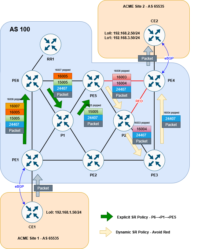
CE1#It works! We can see the traffic following the P6→ P1 → PE5 explicit path, before entering the P4→P5 dynamic path that avoids red using the 15005 label. The 24407 is the VPNv4 advertised from P4 for 192.168.2.0/24.
As proof of concept we can see that tracing to 192.168.3.50 (loopback1) on CE2, whose BGP route does not have a color 10 attribute, is traversing the normal ECMP path we saw at the beginning:
CE1#traceroute 192.168.3.50 source lo0
Type escape sequence to abort.
Tracing the route to 192.168.3.50
VRF info: (vrf in name/id, vrf out name/id)
  1 172.16.1.1 4 msec 2 msec 2 msec
  2 10.10.16.6 [MPLS: Labels 16004/24409 Exp 0] 5 msec 4 msec
    10.10.12.2 [MPLS: Labels 16004/24409 Exp 0] 8 msec
  3 10.10.57.5 [MPLS: Labels 16004/24409 Exp 0] 4 msec
    10.10.56.5 [MPLS: Labels 16004/24409 Exp 0] 5 msec 4 msec
  4 10.10.45.4 [MPLS: Label 24409 Exp 0] 4 msec 4 msec
    10.10.48.4 [MPLS: Label 24409 Exp 0] 3 msec
  5 172.16.2.2 4 msec *  4 msec
CE1#
Here is the final diagram to visualise the result:
So that’s it! There are a lot of different options that SR allows us to use in order to steer traffic intelligently and smoothly across a network. This lab has shown us but one of the methods at our disposal. Further steps might be to implement PCEP for increased scalabilty or introduce more dynamic routing options like performance-measurement – but I’ll leave this variation for a possible later blog.
Thanks so much for reading. Let me know what you think or if you have any comments. Until next time.
The Label Switched Path Not Taken
With the increased introduction of Segment Routing as the label distribution method used by Service Providers, there will inevitably be clashes with the tried and true LDP protocol. Indeed, interoperation between SR and LDP is one of the most important features to consider when introducing SR into a network. But what happen if there is no SR-LDP interoperation to be had? This is definitely the case for IPv6, since LDP for IPv6 is, more often than not, non-existent. This is exactly what this quirk will explore. More specifically, it explores how two different vendors, namely Cisco and Arista, tackle an LSP problem involving native IPv6 MPLS2IP forwarding.
I’ll begin by showing the topology and then give an example of how basic IPv4 SR to LDP interoperation works. We’ll then look at a similar scenario using IPv6 and explore how each vendor behaves. There is no “right answer” to this situation, as neither vendor violates any RFC (at least none that I can find), but it is an interesting exploration of how each approach the same problem.
Setup
I’ll start with a disclaimer, in that this quirk applies to the following software versions in a lab environment:
- Cisco IOS-XR 6.5.3
- Arista 4.25.2F
There is nothing I have seen in either Release Notes, or real world deployments that would make me think that the behaviour described here wouldn’t be the same on the latest releases – but it’s worth keeping in mind. With that said, let’s look at the setup…
The topology we will look at is as follows:

An EVE-NG lab and the base configs can be downloaded here:
The EVE lab has all interfaces unshut. The goal here is for the CE subnets to reach each other. To accomplish this R1 and R6 will run BGP sessions between their loopbacks. In this state, IPv6 forwarding will be broken – but we’ll explore that as we go!
I’ve made the network fairly straightforward to allow us to focus on the quirk. Every device except for R5 runs SR with point-to-point L2 ISIS as the underlaying IGP. The SRGB base is 17000 on all devices. The IPv4 Node SID for each router is its router number. The IPv6 Node SID is the router number plus 600. R5 is an LDP only node and as such, will need a mapping server to advertise it’s node-SID throughout the network – R6 fulfils this role.
To explore the quirk, we will look at forwarding from R1 to R6, loopback-to-loopback. Notice that R3 (a Cisco) and R4 (an Arista) sit on the SR/LDP boundary. IPv4 will be looked at first, to help explain the interoperation between SR and LDP. Once that is done, I’ll demonstrate how each vendor handles IPv6 forwarding differently, which results in forwarding problems.
For now we won’t look at the PE-CE BGP sessions since without the iBGP sessions, our core control plan is broken.
To get the lay of the land let’s check the config on R6 (our destination) and make sure R1’s LFIB is configured correctly.
RP/0/RP0/CPU0:R6#sh run router isis
Wed Nov 23 00:04:51.370 UTC
router isis LAB
 is-type level-2-only
 net 49.0100.1111.1111.0006.00
 log adjacency changes
 address-family ipv4 unicast
  metric-style wide
  advertise passive-only
  segment-routing mpls sr-prefer
  segment-routing prefix-sid-map advertise-local
 !
 address-family ipv6 unicast
  metric-style wide
  advertise passive-only
  segment-routing mpls sr-prefer
 !
 interface Loopback0
  passive
  address-family ipv4 unicast
   prefix-sid absolute 17006
  !
  address-family ipv6 unicast
   prefix-sid absolute 17606
  !
 !
 interface GigabitEthernet0/0/0/3
  point-to-point
  address-family ipv4 unicast
  !
  address-family ipv6 unicast
  !
 !
!
RP/0/RP0/CPU0:R6#sh run segment-routing
Wed Nov 23 00:05:13.681 UTC
segment-routing
 global-block 17000 23999
 mapping-server
  prefix-sid-map
   address-family ipv4
    10.1.1.5/32 5 range 1
   !
  !
 !
!
RP/0/RP0/CPU0:R6#
The same SRGB is configured on all devices. We can see that R6 has SID index 6 for its IPv4 loopback and index 606 for its IPv6 loopback.
With these two pieces of information, we’d expect the CEF table for R1 to use 17006 and 17606 to forward to R6s IPv4 and IPv6 loopbacks respectively….
RP/0/RP0/CPU0:R1#show cef ipv4 10.1.1.6/32
Wed Nov 23 00:11:57.523 UTC
10.1.1.6/32, version 35, labeled SR, internal 0x1000001 0x83 (ptr 0xde0be70) [1], 0x0 (0xdfcd3a8), 0xa28 (0xe4dc2e8)
 Updated Nov 22 17:34:26.975
 remote adjacency to GigabitEthernet0/0/0/0
 Prefix Len 32, traffic index 0, precedence n/a, priority 1
   via 10.1.2.2/32, GigabitEthernet0/0/0/0, 6 dependencies, weight 0, class 0 [flags 0x0]
    path-idx 0 NHID 0x0 [0xecbd140 0x0]
    next hop 10.1.2.2/32
    remote adjacency
     local label 17006      labels imposed {17006}
RP/0/RP0/CPU0:R1#show cef ipv6 2001:1ab::6/128
Wed Nov 23 00:11:59.542 UTC
2001:1ab::6/128, version 32, labeled SR, internal 0x1000001 0x82 (ptr 0xe0db6ac) [1], 0x0 (0xe29a428), 0xa28 (0xe4dc268)
 Updated Nov 22 17:34:26.976
 remote adjacency to GigabitEthernet0/0/0/0
 Prefix Len 128, traffic index 0, precedence n/a, priority 1
   via fe80::5200:ff:fe03:3/128, GigabitEthernet0/0/0/0, 6 dependencies, weight 0, class 0 [flags 0x0]
    path-idx 0 NHID 0x0 [0xd2656a0 0x0]
    next hop fe80::5200:ff:fe03:3/128
    remote adjacency
     local label 17606      labels imposed {17606}
RP/0/RP0/CPU0:R1#
So far so good. Let’s start with a full IPv4 traceroute and see how SR interoperates with LDP.
IPv4 connectivity and LDP interoperability
We’ll look at this by first examining Cisco’s behaviour, so let’s shutdown the R2 to R4 Arista link (Gi0/0/0/2)…
RP/0/RP0/CPU0:R2(config)#int GigabitEthernet 0/0/0/2
RP/0/RP0/CPU0:R2(config-if)#shut
RP/0/RP0/CPU0:R2(config-if)#commit
From here, we do a basic traceroute:
RP/0/RP0/CPU0:R1#traceroute 10.1.1.6 source lo0
Wed Nov 23 00:13:59.116 UTC

Type escape sequence to abort.
Tracing the route to 10.1.1.6

 1  10.1.2.2 [MPLS: Label 17006 Exp 0] 152 msec  142 msec  135 msec
 2  10.2.3.3 [MPLS: Label 17006 Exp 0] 142 msec  148 msec  146 msec
 3  10.3.5.5 [MPLS: Label 18 Exp 0] 140 msec  137 msec  135 msec
 4  10.5.6.6 148 msec  *  126 msec
RP/0/RP0/CPU0:R1#
Here’s a visual diagram of what is happening:

Let’s look a bit closer at what is happening here. How does R3 program its LFIB? For segment routing the LFIB programming works like this:
- Local label: The Node SID + the SRGB Base (in our case 6 + 17000 = 17006)
- Outbound label: The Node SID + the SRGB Base of the next-hop for that prefix
Now if the next-hop was SR capable, and the SRGB was contiguous through the domain (e.g. it was 17000 everywhere), the outbound label would be 17006 as well. But here, R5 is not SR capable. It isn’t advertising any SR TLV information in its ISIS LDPUs. But it does have LDPs sessions with all of its neighbors, including R3.
R5#sh mpls ldp neighbor | inc Peer|Gig
    Peer LDP Ident: 10.1.1.4:0; Local LDP Ident 10.1.1.5:0
	  GigabitEthernet1, Src IP addr: 10.4.5.4
    Peer LDP Ident: 10.1.1.6:0; Local LDP Ident 10.1.1.5:0
	  GigabitEthernet3, Src IP addr: 10.5.6.6
    Peer LDP Ident: 10.1.1.3:0; Local LDP Ident 10.1.1.5:0
	  GigabitEthernet2, Src IP addr: 10.3.5.3
R5#
As you might be able to predict, this is where the SR to LDP interoperation comes into play. R5 will have advertised its local label for 10.1.1.6 to R3.
RP/0/RP0/CPU0:R3#sh mpls ldp ipv4 bindings 10.1.1.6/32
Wed Nov 23 00:14:23.126 UTC
10.1.1.6/32, rev 17
        Local binding: label: 16300
        Remote bindings: (1 peers)
            Peer                Label
            -----------------   ---------
            10.1.1.5:0          18
RP/0/RP0/CPU0:R3#
So R5 will use this instead! The basic principle is as follows:
Interworking is achieved by replacing an unknown outbound label from one protocol by a valid outgoing label from another protocol.
SR is basically “inheriting” from LDP. R3’s forwarding table looks as follows:
RP/0/RP0/CPU0:R3#sh mpls forwarding labels 17006
Wed Nov 23 00:26:02.364 UTC
Local  Outgoing    Prefix             Outgoing     Next Hop        Bytes
Label  Label       or ID              Interface                    Switched
------ ----------- ------------------ ------------ --------------- ------------
17006  18          SR Pfx (idx 6)     Gi0/0/0/2    10.3.5.5        3808
RP/0/RP0/CPU0:R3#
The local label is the SR label and the outbound label is the LDP label of 18. You can see from the traceroute that this indeed the label used.
RP/0/RP0/CPU0:R1#traceroute 10.1.1.6 source lo0
Wed Nov 23 00:13:59.116 UTC

Type escape sequence to abort.
Tracing the route to 10.1.1.6

 1  10.1.2.2 [MPLS: Label 17006 Exp 0] 152 msec  142 msec  135 msec
 2  10.2.3.3 [MPLS: Label 17006 Exp 0] 142 msec  148 msec  146 msec
 3  10.3.5.5 [MPLS: Label 18 Exp 0] 140 msec  137 msec  135 msec
 4  10.5.6.6 148 msec  *  126 msec
RP/0/RP0/CPU0:R1#
NB. I’ve missed a couple of details here, namely how LDP to SR works in the opposite direction in conjunction with mapping server statements. These don’t directly relate to our quirk here, since we’re focusing on R1 to R6 traffic, but I’d recommend reading the Segment Routing Book Series found on segment-routing.net to get the full details of SR/LDP interoperability.
Now that we’ve verified forwarding through the Cisco, we’ll switch to the Arista path to ensure that the behaviour is identical. First we’ll shutdown R2’s uplink to R3 (Gi0/0/0/1) and unshut its uplink to R4 (Gi0/0/0/2), before rerunning the traceroute:
RP/0/RP0/CPU0:R2(config)#int GigabitEthernet 0/0/0/2
RP/0/RP0/CPU0:R2(config-if)#no shut
RP/0/RP0/CPU0:R2(config-if)#int GigabitEthernet 0/0/0/1
RP/0/RP0/CPU0:R2(config-if)#shut
RP/0/RP0/CPU0:R2(config-if)#commit
Wed Nov 23 00:40:25.104 UTC
LC/0/0/CPU0:Nov 23 00:40:25.219 UTC: ifmgr[270]: %PKT_INFRA-LINK-3-UPDOWN : Interface GigabitEthernet0/0/0/2, changed state to Down
LC/0/0/CPU0:Nov 23 00:40:25.318 UTC: ifmgr[270]: %PKT_INFRA-LINK-3-UPDOWN : Interface GigabitEthernet0/0/0/2, changed state to Up
RP/0/RP0/CPU0:R2(config-if)#
RP/0/RP0/CPU0:R1#traceroute 10.1.1.6 source lo0
Wed Nov 23 00:41:12.857 UTC

Type escape sequence to abort.
Tracing the route to 10.1.1.6

 1  10.1.2.2 [MPLS: Label 17006 Exp 0] 57 msec  54 msec  56 msec
 2   *  *  *
 3  10.4.5.5 [MPLS: Label 18 Exp 0] 60 msec  53 msec  51 msec
 4  10.5.6.6 60 msec  *  62 msec
RP/0/RP0/CPU0:R1#
Success! It’ using the LDP label 18 just as before and if we run some of the Arista CLI commands we see similar inheritance behaviour to the Cisco:
R4#show mpls lfib route | begin 10.1.1.6/32
 IL  17006    [1], 10.1.1.6/32
                via M, 10.4.5.5, swap 18
                 payload autoDecide, ttlMode uniform, apply egress-acl
                 interface Ethernet1
<<snip>>
Here’s the diagram:
So IPv4 looks solid. If no SR, then fall back to LDP. But what happens if we use IPv6? There is no LDP for IPv6. More importantly though… what should happen? Let’s explore what both vendors do and then you can make up your own mind.
IPv6 Connectivity and LDP
Let’s flip back to Cisco and see what the traceroute looks like:
RP/0/RP0/CPU0:R2(config-if)#int GigabitEthernet 0/0/0/2
RP/0/RP0/CPU0:R2(config-if)#shut
RP/0/RP0/CPU0:R2(config-if)#int GigabitEthernet 0/0/0/1
RP/0/RP0/CPU0:R2(config-if)#no shut
RP/0/RP0/CPU0:R2(config-if)#commit
Wed Nov 23 00:49:08.711 UTC
LC/0/0/CPU0:Nov 23 00:49:08.787 UTC: ifmgr[270]: %PKT_INFRA-LINK-3-UPDOWN : Interface GigabitEthernet0/0/0/1, changed state to Down
LC/0/0/CPU0:Nov 23 00:49:08.837 UTC: ifmgr[270]: %PKT_INFRA-LINK-3-UPDOWN : Interface GigabitEthernet0/0/0/1, changed state to Up
RP/0/RP0/CPU0:R2(config-if)#
RP/0/RP0/CPU0:R1#traceroute ipv6 2001:1ab::6 source lo0
Wed Nov 23 00:50:51.770 UTC
Type escape sequence to abort.
Tracing the route to 2001:1ab::6
1 2001:1ab:1:2::2 [MPLS: Label 17606 Exp 0] 261 msec 48 msec 47 msec
2 2001:1ab:2:3::3 [MPLS: Label 17606 Exp 0] 52 msec 33 msec 46 msec
3 2001:1ab:3:5::5 50 msec 49 msec 48 msec
4 2001:1ab::6 105 msec 86 msec 88 msec
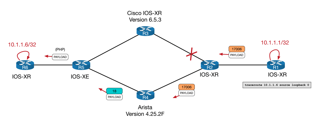
RP/0/RP0/CPU0:R1#Here we see something a bit unexpected. R3 is actually popping the top label and forwarding it on natively:

But why is this? If you have an incoming label but no outgoing label isn’t that, by definition, a broken LSP? So why does Cisco forward the packet natively?
Well, for this I’m going to take a quote from the Segment Routing Part 1 book (again found on segment-routing.net). Granted this isn’t an RFC, but it does a good job of explaining the Cisco IOS-XR behaviour.
If the incoming packet has a single label … (the label has the End of Stack (EOS) bit set to indicate it is the last label), then the label is removed and the packet is forwarded as an IP packet. If the incoming packet has more than one label … then the packet is dropped and this would be the erroneous termination of the LSP that we referred to previously.
Segment Routing, Part 1 by by Clarence Filsfils , Kris Michielsen , et al.
What’s happening with R3 here is MPLS2IP behaviour (since the LSP is ending and the packet is being forwarded natively). Based on the above, I believe the rule that R3 is following when deciding how to forward the incoming packet works like this:
- If there is one SR label with EoS bit set, then Forward on natively
- Else, treat as broken LSP and drop
Both CEF and the LFIB reflect this behaviour with Unlabelled as the outgoing label:
RP/0/RP0/CPU0:R3#show mpls forwarding labels 17606
Wed Nov 23 00:55:21.324 UTC
Local  Outgoing    Prefix             Outgoing     Next Hop        Bytes
Label  Label       or ID              Interface                    Switched
------ ----------- ------------------ ------------ --------------- ------------
17606  Unlabelled  SR Pfx (idx 606)   Gi0/0/0/2    fe80::5200:ff:fe05:1   \
                                                                   778986
RP/0/RP0/CPU0:R3#sh cef mpls local-label 17606 EOS
Wed Nov 23 00:55:27.537 UTC
Label/EOS 17606/1, version 27, labeled SR, internal 0x1000001 0x82 (ptr 0xd3575b0) [1], 0x0 (0xe3a44a8), 0xa20 (0xe4dc3a8)
 Updated Jan 10 13:37:10.343
 remote adjacency to GigabitEthernet0/0/0/2
 Prefix Len 21, traffic index 0, precedence n/a, priority 1
   via fe80::5200:ff:fe05:1/128, GigabitEthernet0/0/0/2, 8 dependencies, weight 0, class 0 [flags 0x0]
    path-idx 0 NHID 0x0 [0xd576738 0x0]
    next hop fe80::5200:ff:fe05:1/128
    remote adjacency
     local label 17606      labels imposed {None}
But why forwarding if only one label?
I believe that Cisco is making the assumption that if there is only one label, that label is likely to be a transport label. The would imply that the underlying IPv6 address is an endpoint loopback address in the IGP, which any subsequence P router would most likely know. This allows traffic to be forwarded on in brownfield migration scenario similar to our lab.
If there is more that one label, then it would seem prudent to drop it as any underlying labels are likely to be VPN or service labels that the next P router would not understand.
I can’t be sure that this is the reasoning Cisco were going for, but it seems reasonable to me.
Now the we know how Cisco does it, let’s look at how Arista’s tackles the same scenario. Just like with IPv4 we’ll flip the path and retry the traceroute:
RP/0/RP0/CPU0:R2(config)#interface GigabitEthernet 0/0/0/1
RP/0/RP0/CPU0:R2(config-if)#shut
RP/0/RP0/CPU0:R2(config-if)#interface GigabitEthernet 0/0/0/2
RP/0/RP0/CPU0:R2(config-if)#no shut
RP/0/RP0/CPU0:R2(config-if)#commit
Wed Nov 23 00:57:01.906 UTC
LC/0/0/CPU0:Wed Nov 23 00:57:02.486 UTC: ifmgr[270]: %PKT_INFRA-LINK-3-UPDOWN : Interface GigabitEthernet0/0/0/2, changed state to Down
LC/0/0/CPU0:Wed Nov 23 00:57:02.533 UTC: ifmgr[270]: %PKT_INFRA-LINK-3-UPDOWN : Interface GigabitEthernet0/0/0/2, changed state to Up
RP/0/RP0/CPU0:R2(config-if)#
RP/0/RP0/CPU0:R1#traceroute ipv6 2001:1ab::6 source lo0
Wed Nov 23 01:00:12.976 UTC
Type escape sequence to abort.
Tracing the route to 2001:1ab::6
1 * * *
2 * * *
3 * * *
4 * * *
^C
RP/0/RP0/CPU0:R1#
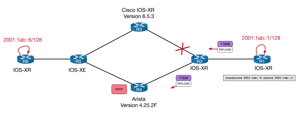
No Network Engineer ever likes to see a broken traceroute. But clearly something isn’t getting through.
Output when looking at the LFIB from Arista starts to give us an idea:
R4#show mpls lfib route 17606
MPLS forwarding table (Label [metric] Vias) - 0 routes
MPLS next-hop resolution allow default route: False
Via Type Codes:
          M - MPLS via, P - Pseudowire via,
          I - IP lookup via, V - VLAN via,
          VA - EVPN VLAN aware via, ES - EVPN ethernet segment via,
          VF - EVPN VLAN flood via, AF - EVPN VLAN aware flood via,
          NG - Nexthop group via
Source Codes:
          G - gRIBI, S - Static MPLS route,
          B2 - BGP L2 EVPN, B3 - BGP L3 VPN,
          R - RSVP, LP - LDP pseudowire,
          L - LDP, M - MLDP,
          IP - IS-IS SR prefix segment, IA - IS-IS SR adjacency segment,
          IL - IS-IS SR segment to LDP, LI - LDP to IS-IS SR segment,
          BL - BGP LU, ST - SR TE policy,
          DE - Debug LFIB

R4#
Unlike Cisco, there is no outgoing entry in the LFIB on the Arista for 17606.
Interestingly though, tracing does work directly from R4 to R6:
R4#traceroute ipv6 2001:1ab::6 source 2001:1ab::4
traceroute to 2001:1ab::6 (2001:1ab::6), 30 hops max, 80 byte packets
 1  2001:1ab:4:5::5 (2001:1ab:4:5::5)  5.145 ms  9.544 ms  10.500 ms
 2  2001:1ab::6 (2001:1ab::6)  95.139 ms  94.834 ms  96.574 ms
R4#
This ping is a case of IP2IP forwarding. Arista, being aware that it has no label for the next-hop, forwards it natively. It’s similar to Cisco, but Cisco have an aforementioned MPLS2IP rule that bridges the two parts.
To begin troubleshooting the Arista, let’s check the basics. We already know that there is no LFIB entry for 17606. We’d expect to see it at the bottom of this table…
R4#show mpls lfib route detail | inc 17
 IP  17001    [1], 10.1.1.1/32
                via M, 10.2.4.2, swap 17001
 IP  17002    [1], 10.1.1.2/32
 IL  17003    [1], 10.1.1.3/32
                via M, 10.4.5.5, swap 17
 IP  17005    [1], 10.1.1.5/32
 IL  17006    [1], 10.1.1.6/32
 IP  17601    [1], 2001:1ab::1/128
                via M, fe80::5200:ff:fe03:5, swap 17601
 IP  17602    [1], 2001:1ab::2/128
                via M, 10.2.4.2, swap 17001
                via M, 10.4.5.5, swap 17
R4#
Perhaps R4 is not getting the correct Segment Routing information. We know from our initial config check that R6 is configured correctly. When SR is enabled on a device (no matter the vendor) an SR-Capability sub-TLV is added under the Router Capability TLV. This essentially signals that it is SR capable as well as various other SR aspects.
We can see that R4 is aware that R6 is SR enabled and gets all of the correct Node-SID information:
R4#sh isis database R6.00-00 detail

IS-IS Instance: LAB VRF: default
  IS-IS Level 2 Link State Database
    LSPID                 Seq Num   Cksum  Life  IS Flags
    R6.00-00              3184      38204  1104  L2 <>
      Remaining lifetime received: 1198 s Modified to: 1200 s
<snip>
      IS Neighbor (MT-IPv6): R5.00               Metric: 10
        Adj-sid: 16312 flags: [ L V F ] weight: 0x0
      Reachability         : 10.1.1.6/32 Metric: 0 Type: 1 Up
        SR Prefix-SID: 6 Flags: [ N ] Algorithm: 0
      Reachability (MT-IPv6): 2001:1ab::6/128 Metric: 0 Type: 1 Up
        SR Prefix-SID: 606 Flags: [ N ] Algorithm: 0
      Router Capabilities: Router Id: 10.1.1.6 Flags: [ ]
        SR Local Block:
          SRLB Base: 15000 Range: 1000
        SR Capability: Flags: [ I V ]
          SRGB Base: 17000 Range: 7000
        Algorithm: 0
        Algorithm: 1
      Segment Binding: Flags: [ ] Weight: 0 Range: 1 Pfx 10.1.1.5/32
        SR Prefix-SID: 5 Flags: [ ] Algorithm: 0

R4#show isis segment-routing prefix-segments vrf all

System ID: 1111.1111.0004			Instance: 'LAB'
SR supported Data-plane: MPLS			SR Router ID: 10.1.1.4

Node: 10     Proxy-Node: 1      Prefix: 0       Total Segments: 11

Flag Descriptions: R: Re-advertised, N: Node Segment, P: no-PHP
                   E: Explicit-NULL, V: Value, L: Local
Segment status codes: * - Self originated Prefix, L1 - level 1, L2 - level 2, ! - SR-unreachable,
                      # - Some IS-IS next-hops are SR-unreachable
   Prefix                      SID Type       Flags                   System ID       Level Protection
   ------------------------- ----- ---------- ----------------------- --------------- ----- ---
<snip>
   2001:1ab::1/128             601 Node       R:0 N:1 P:0 E:0 V:0 L:0 1111.1111.0001  L2    unprotected
   2001:1ab::2/128             602 Node       R:0 N:1 P:0 E:0 V:0 L:0 1111.1111.0002  L2    unprotected
   2001:1ab::3/128             603 Node       R:0 N:1 P:0 E:0 V:0 L:0 1111.1111.0003  L2    unprotected
*  2001:1ab::4/128             604 Node       R:0 N:1 P:0 E:0 V:0 L:0 1111.1111.0004  L2    unprotected
   2001:1ab::6/128             606 Node       R:0 N:1 P:0 E:0 V:0 L:0 1111.1111.0006  L2    unprotected
R4#
So far so good. But why no LFIB entry? Well, for us to understand what is happening here, we need to understand how Arista programs its LFIB.
When Arista forwards using Segment Routing, the entry is first assigned in this SR-bindings table and only then does it enters the LFIB. We can see it makes it into the SR-bindings table:
R4#show mpls segment-routing bindings ipv6
2001:1ab::1/128
   Local binding:  Label: 17601
   Remote binding: Peer ID: 1111.1111.0002, Label: 17601
2001:1ab::2/128
   Local binding:  Label: 17602
   Remote binding: Peer ID: 1111.1111.0002, Label: imp-null
2001:1ab::3/128
   Local binding:  Label: 17603
   Remote binding: Peer ID: 1111.1111.0002, Label: 17603
2001:1ab::4/128
   Local binding:  Label: imp-null
   Remote binding: Peer ID: 1111.1111.0002, Label: 17604
2001:1ab::6/128
   Local binding:  Label: 17606
   Remote binding: Peer ID: 1111.1111.0002, Label: 17606
R4#
But why does it not then enter the LFIB? I believe that what is happening here is that it fails to program the LFIB based on the rules outlined above, namely:
- Local label: The Node SID + the SRGB Base (in our case 6 + 17000 = 17006)
- Outbound label: The Node SID + the SRGB Base of the next-hop for that prefix
The outbound label can’t be determined since the IGP network hop to 2001:1ab::6 is R5, a device that isn’t running SR. With no LDP to inherit from (since there is not LDP for IPv6) and without a special rule to forward natively (like Cisco has) the LFIB is never programmed and the packet is dropped!
Note that in the above SR-bindings table there are Remote Bindings. But these are all from R2 (the Peer ID of 1111.1111.0002 is the ISIS the system ID of R2) which is not the IGP next hop.
NB. If you are doing packet traces on a physical appliance, the “show cpu counters queue summary” command will reveal the “CoppSystemMplsLabelMiss” Packets incrementing as traffic is dropped during the traceroute. I’ve omitted is here as the command won’t work in a virtual lab environment.
So who is correct?
The obvious question at this point becomes, who is correct? Yes the traffic gets through the Cisco, but isn’t it kind of violating the principle of a broken LSP. After-all if LDP goes down between two devices in an SP core, don’t we want to avoid using that link? Isn’t that the idea behind things like LDP-IGP Sync? What if Cisco forwards an MPLS2IP packet natively and the next hop sends the packet somewhere unintended? I imagine situations like this would be rare, but maybe Arista are right playing it safe and dropping it?
I’ve tried to find an authoritative source by going on an RFC hunt – with hope of using it to determine what behaviour ought to be followed.
Unfortunately, I couldn’t find a direct reference in any RFC. The closest reference I could get was a brief mention in RFC 8661 in the MPLS2MPLS, MPLS2IP, and IP2MPLS Coexistence section.
The same applies for the MPLS2IP forwarding entries. MPLS2IP is the forwarding behavior where a router receives a labeled IPv4/IPv6 packet with one label only, pops the label, and switches the packet out as IPv4/IPv6.
RFC 8661 Section 2.1
This does little more than reference the existence of MPLS2IP forwarding. It certainly doesn’t tell us the correct behaviour. If anyone knows of an authority to resolve this, please feel free to let me know! Unfortunately at this stage, each vendors appears free to program whatever forwarding behaviour they like.
To that end, I put it to you, what do you think is the best behaviour in scenarios like this?
My personal preference is the Cisco option, because it allows for brown field migrations like those that we encountered. Without an IPv6 label distribution tool, or without reverting to 6PE, this behaviour I believe is warranted. The most likely worst case scenario is that the next hop router will simple discard the packet due to not having a route – however I concede there might be scenarios where this could be problematic.
Until there is consistency between vendors we’ll need ways to work around scenarios like this. Let’s take a look at a few.
Solutions
Sadly most of the solutions to this are suitably dull. They either involve removing the IPv6 next hop, the label, or both…
Remove the IPv6 Node SID
This is perhaps the simplest option. By removing the IPv6 node SID from R6, R1 would have no entry for R6 in its LFIB and as a result would forward the traffic natively. We can demonstrate this by doing the following:
! The link via the Cisco device R3 is admin down to make sure traffic travels via the Arista
RP/0/RP0/CPU0:R6(config)#router isis LAB
RP/0/RP0/CPU0:R6(config-isis)# interface Loopback0
RP/0/RP0/CPU0:R6(config-isis-if)#  address-family ipv6 unicast
RP/0/RP0/CPU0:R6(config-isis-if-af)#no prefix-sid absolute 17606
RP/0/RP0/CPU0:R6(config-isis-if-af)#commit
Wed Nov 23 01:10:43.103 UTC
RP/0/RP0/CPU0:Wed Nov 23 01:10:45.432 UTC: config[67901]: %MGBL-CONFIG-6-DB_COMMIT : Configuration committed by user 'user1'. Use 'show configuration commit changes 1000000015' to view the changes.
RP/0/RP0/CPU0:R6(config-isis-if-af)#RP/0/RP0/CPU0:Wed Nov 23 01:10:47.089 UTC: bgp[1060]: %ROUTING-BGP-5-ADJCHANGE_DETAIL : neighbor 2001:1ab::1 Up (VRF: default; AFI/SAFI: 2/1) (AS: 100)
RP/0/RP0/CPU0:R6(config-isis-if-af)#
! note the native forwardingRP/0/RP0/CPU0:R1#traceroute 2001:1ab::6 source 2001:1ab::1
Wed Nov 23 01:11:02.802 UTC
Type escape sequence to abort.
Tracing the route to 2001:1ab::6
1 2001:1ab:1:2::2 79 msec 4 msec 3 msec
2 2001:1ab:2:4::4 6 msec 5 msec 5 msec
3 2001:1ab:4:5::5 8 msec 8 msec 7 msec
4 2001:1ab::6 12 msec 11 msec 9 msec
RP/0/RP0/CPU0:R1#Weight out the Arista link
I’ll only mention this in passing, since, whilst is does allow the Arista to remain live in the network for IPv4 traffic, weighting the link out is more akin to avoiding the problem rather than solving it. Here’s an example of changing the ISIS metric.
R4(config)#int eth2
R4(config-if-Et2)#isis ipv6 metric 9999
R4(config-if-Et2)#int eth4
R4(config-if-Et4)#isis ipv6 metric 9999
Reverting to 6PE
You might ask why this lab choses to use native BGP IPv6 in the first place, rather than use 6PE. Other than wanting to future proof the network and utilise all the benefits that come with SR, the real world scenario upon which is blog is loosely based involved 6PE bug. Basically a 6PE router was allocating one label per IPv6 prefix rather than a null label. This resulted in label exhaustion issues on the device in question. The details are beyond the scope of this blog but provides a little context. Regardless, if we use 6PE, the next hops are now IPv4 loopbacks. This allows the normal SR/LDP interoperability to take place as outlined above. Here is the basic config and verification:
RP/0/RP0/CPU0:R1(config)#router bgp 100
RP/0/RP0/CPU0:R1(config-bgp)#address-family ipv6 unicast
RP/0/RP0/CPU0:R1(config-bgp-af)#allocate-label all
RP/0/RP0/CPU0:R1(config-bgp-af)#exit
RP/0/RP0/CPU0:R1(config-bgp)#neighbor 10.1.1.6
RP/0/RP0/CPU0:R1(config-bgp-nbr)#address-family ipv6 labeled-unicast
! similar commands done on R6 not shown here

RP/0/RP0/CPU0:R1#sh bgp ipv6 labeled-unicast
Wed Nov 23 01:17:39.800 UTC
BGP router identifier 10.1.1.1, local AS number 100
BGP generic scan interval 60 secs
Non-stop routing is enabled
BGP table state: Active
Table ID: 0xe0800000   RD version: 4
BGP main routing table version 4
BGP NSR Initial initsync version 2 (Reached)
BGP NSR/ISSU Sync-Group versions 0/0
BGP scan interval 60 secs

Status codes: s suppressed, d damped, h history, * valid, > best
              i - internal, r RIB-failure, S stale, N Nexthop-discard
Origin codes: i - IGP, e - EGP, ? - incomplete
   Network            Next Hop            Metric LocPrf Weight Path
*> 2001:cafe:1::/64   2001:db8:1::1            0             0 65489 i
*>i2001:cafe:2::/64   10.1.1.6                 0    100      0 65489 i

Processed 2 prefixes, 2 paths
RP/0/RP0/CPU0:R1#
CE1#traceroute 2001:cafe:2::1 source 2001:cafe:1::1
Type escape sequence to abort.
Tracing the route to 2001:CAFE:2::1
1 2001:DB8:1:: 4 msec 3 msec 1 msec
2 * * *
3 * * *
4 ::FFFF:10.4.5.5 [MPLS: Labels 20/16302 Exp 0] 15 msec 14 msec 26 msec
5 * * *
6 2001:DB8:2::1 15 msec 14 msec 10 msec
CE1#Implement Segment Routing using IPv6 Headers
I’ll only mention this is passing as I’ve not seen this implemented in the wild and am not sure if my lab environment would support it. Suffice it to say that if this could be implemented, it would remove the need for LDP labels entirely.
6PE from P router to PE
I toyed with this idea out of curiosity more than anything else. I’d not recommend this for a real world deployment, but the general idea is as follows:
- Run 6PE between the trouble P router (in our case R4) and the destination PE router (R6)
- The PE router would advertise its IPv6 loopback over the 6PE session.
- The P router would filter it’s 6PE session to only accept PE loopback addresses
- The P router would set the Administrative Distance of the IGP to be 201, so it would prefer the iBGP AD of 200 to reach the end point.
The idea is that as soon as the traffic reaches the P router, the next hop to the IPv6 end point is not seen via the IGP but rather, via the 6PE session. The result would be that the incoming IPv6 SR label is replace with two labels – the bottom label is the 6PE label for the IPv6 endpoint address, the top label is the transport address for the IPv4 address of the 6PE peer (and SR to LDP interoperability can take over here). This might be scalable if the P router we running 6PE to the all the PEs via a router reflector and an inbound route-map only allowed in their next-hop loopbacks.
To put this in diagram form, it would look like this:
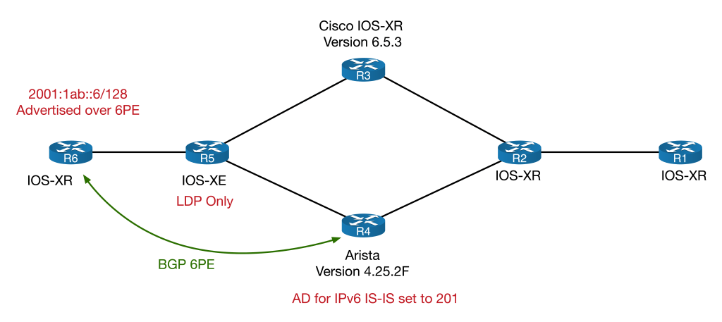
Unfortunately my virtual Arista didn’t support 6PE. I did test the principle on my Cisco P device (R3) and it seemed to work. Here is the basic config and verification:
! R3's BGP config
router bgp 100
 bgp router-id 10.1.1.3
 bgp log neighbor changes detail
 address-family ipv6 unicast
  allocate-label all
 !
 neighbor 10.1.1.6
  remote-as 100
  update-source Loopback0
  address-family ipv6 labeled-unicast
   route-policy ONLY-PEs in
  !
 !
!
route-policy ONLY-PEs
  if destination in (2001:1ab::6/128) then
    pass
  else
    drop
  endif
end-policy
! R6's BGP config
router bgp 100
 bgp router-id 10.1.1.6
 address-family ipv6 unicast
  network 2001:1ab::6/128
  allocate-label all
 !
!
 neighbor 10.1.1.4
  remote-as 100
  update-source Loopback0
  address-family ipv6 labeled-unicast
 !
!
R3 now sees next hop via 6PE BGP session with 6PE label:
RP/0/RP0/CPU0:R3#sh route ipv6 2001:1ab::6
Wed Nov 23 01:21:43.710 UTC

Routing entry for 2001:1ab::6/128
  Known via "bgp 100", distance 200, metric 0, type internal
  Installed Nov  23 01:19:01.151 for 00:02:23
  Routing Descriptor Blocks
    ::ffff:10.1.1.6, from ::ffff:10.1.1.6
      Nexthop in Vrf: "default", Table: "default", IPv4 Unicast, Table Id: 0xe0000000
      Route metric is 0
  No advertising protos.
RP/0/RP0/CPU0:R3#sh bgp ipv6 labeled-unicast 2001:1ab::6
Wed Nov 23 01:21:45.081 UTC
BGP routing table entry for 2001:1ab::6/128
Versions:
  Process           bRIB/RIB  SendTblVer
  Speaker                  3           3
Last Modified: Nov  23 01:18:58.980 for 00:01:54
Paths: (1 available, best #1)
  Not advertised to any peer
  Path #1: Received by speaker 0
  Not advertised to any peer
  Local
    10.1.1.6 (metric 20) from 10.1.1.6 (10.1.1.6)
      Received Label 16300
      Origin IGP, metric 0, localpref 100, valid, internal, best, group-best, labeled-unicast
      Received Path ID 0, Local Path ID 1, version 3
RP/0/RP0/CPU0:R3#
Traceroute confirms 6PE path:
RP/0/RP0/CPU0:R1#traceroute 2001:1ab::6 source 2001:1ab::1
Wed Nov 23 01:23:24.423 UTC

Type escape sequence to abort.
Tracing the route to 2001:1ab::6

 1  2001:1ab:1:2::2 [MPLS: Label 17606 Exp 0] 38 msec 6 msec 5 msec
 2  2001:1ab:2:3::3 [MPLS: Label 17606 Exp 0] 6 msec 5 msec 5 msec
 3  ::ffff:10.3.5.5 [MPLS: Labels 18/16300 Exp 0] 5 msec 5 msec 6 msec
 4  2001:1ab::6 7 msec 6 msec 6 msec
RP/0/RP0/CPU0:R1#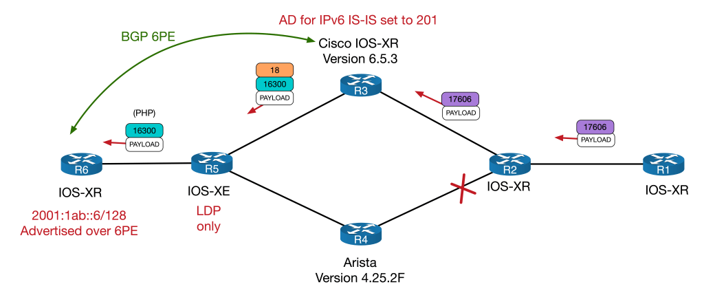
18 is R5’s LDP label for 10.1.1.6 and 16300 is the 6PE label for 2001:1ab::6. Whilst this technically would work, it would also mean that R3 would always use 6PE to any IPv6 endpoint it received over the 6LU session – it would however, allow the IPv6 node SID and native IPv6 session to remain in place.
Again, this was a thought exercise more than anything else – I wouldn’t recommend this for a live deployment without a lot more testing.
Conclusion
Here, we’ve seen an unexpected scenario whereby Cisco forwards single labelled SR packets natively, but Arista treats it as a broken LSP, as it arguably is. This causes problem for MPLS2IP forwarding for IPv6 packets in a brownfield migration. Ultimately it comes down the way to which each vendor choses to implement their LFIBs. At time of writing, the only real solution are to remove the IPv6 next-hop, the label or both – however it will be interesting to see moving forwarding if SRv6 or perhaps even some inter-vendor consensus could resolve this interesting quirk. Thanks so much for reading. Thoughts and comments are welcome as always.
TI-LFA FTW!
Having fast convergence times is one of most important aspects of running any Service Provider network. But perhaps more important is making sure that you actual have the necessary backup paths in the first place.
This quirk explores a network within which neither Classic Loop Free Alternate (LFA) nor Remote-LFA (R-LFA) provide complete backup coverage, and how Segment Routing can solve this using a technology called Topology Independent Loop Free Alternate (or TI-LFA).
This blog comes with a downloadable EVE-NG lab that can be found here. It is configured with the final TI-LFA and SR setup, but I’ll provide the configuration examples for both Classic-LFA and R-LFA as we go. We’ll just look at link protection in this post, but the principle for node and SRLG protection is similar.
I’ll assume anyone reading is well versed in the IGP + LDP Service Provider core model but will give a whistle stop introduction to Segment Routing for those who haven’t run into it yet…
Segment Routing – A Brief Introduction
Segment Routing (or SR) is one of the most exciting new technologies in the Service Provider world. On the face of it, it looks like “just another way to communicate labels” but once you dig into it, you’ll realise how powerful it can be.
This introduction will be just enough to get you to understand this post if you’ve never used SR before. I highly recommend checking out segment-routing.net for more information.
The best way to introduce SR is to compare it to LDP. So to that end, here’s a basic diagram as a reminder of how LDP works:
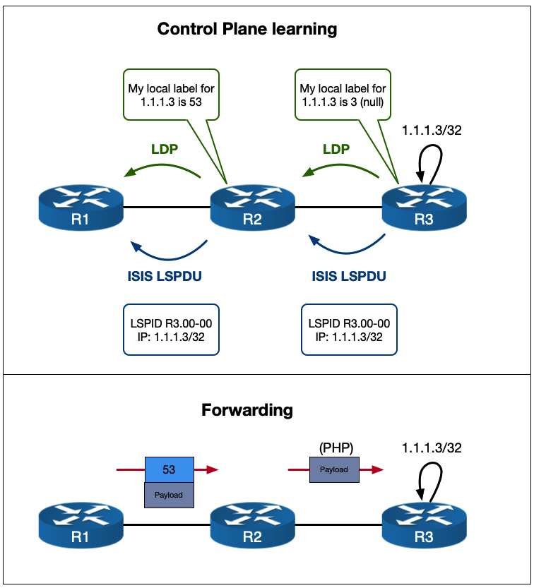
R3 is advertising its 1.1.1.3/32 loopback via ISIS and LDP communicates label information. This should hopefully be very familiar.
So how does SR differ?
Well, the difference is in how the label is communicated. Instead of using an extra protocol, like LDP, the label information is carried in the IGP itself. In the case of ISIS, it uses TLVs. In the case of OSPF it uses opaque LSAs (which are essentially a mechanism for carrying TLVs in and of themselves).
This means that instead of each router allocating is own label for every single prefix in its IGP routing table and then advertising these to their neighbors using multiple LDP sessions, the router that sources the prefix advertises its label information inside its IGP update packets. Only the source router actually does any allocating.
Before I show you a diagram, let’s get slightly technical about what SR is…
Segment Routing is defined as … “a source-based routing paradigm that uses stacks of instructions – referred to as Segments – to forward packets”. This might seem confusing, but basically Segments are MPLS Labels (they can also be IPv6 headers but we’ll just deal with MPLS labels here). Each label in a stack can be thought of as an instruction that tells the router what do with the packet.
There are two types of Segments (or instructions) we need to be concerned with in this post. Node-SIDs and Adj-SIDs.
- A Node-SID in a Service Provider network typically refers to a loopback address of a router that something like BGP would use as the next-hop (e.g. it puts the self in next-hop-self). This is analogous to the LDP label for a given IGP prefix that each route in an ISP core would assign. The “instruction” for a Node-SID is forward this packet on to the prefix along your best ECMP path for it.
- An Adj-SID represents a routers IGP neighborship. An Adj-SID has the “instruction” of forwarding this packet out of the interface toward this neighbor.
So how are these allocated and adverted?
Like I said before, they use the TLVs (or opaque LSAs) of the IGPs involved. But the advertisements of Adj-SIDs and Node-SIDs do differ slightly…
Adj-SIDs are (by default) automatically allocated from the default MPLS label pool (the same pool used to allocate LDP labels) and are simply advertised inside the TLV “as is”. There is more than one type of Adj-SIDs for each IGP neighbor… they come in both protected/unprotected and IPv4/IPv6 flavours. This post will only deal with IPv4 unprotected, so don’t worry about the others for now.
The Node-SID is a little more complicated. It is statically assigned under the IGP config and comes from a reserved label range called the SRGB or Segment Routing Global Block. This is a different block from the default MPLS one and the best way to understand it is to put it in context…
Let’s say your SRGB is 17000-18999. This is a range of 2000 labels. And let’s say that each router in the network get’s a Node-SID based on its router number (e.g. R5 gets Node-SID 17005 etc..). Well when a router advertises this information inside the TLV, it breaks it up into several key bits of information:
• The Prefix itself – a /32 when dealing with IPv4.
• A globally significant Index – this is just a number. In our case R5 gets index 5 and so on…
• The locally significant SRGB Base value – the first label in the Segment Routing label range. In our case the SRGB base is 17000.
• A locally significant Range value stating how big the SRGB is – for us it’s 2000
So for any given router its overall SRGB is the Base plus the Range. And because both the Base and the Range are locally significant, so is the SRGB.
What does this local significance mean?
Well it obviously means that it can differ one device to another… so when I said above “Let’s say your SRGB is 17000-18999″ I’ve assumed that all devices in the network have the same SRGB (and by extension the same Base and Range) configured. Again to best understand this, let’s continue within our current context…
Just like LDP each router installs an In and Out label in the LFIB for each prefix:
• The In label is the Index of that prefix plus its own local SRGB.
• The Out label is the Index plus the downstream neighbor’s SRGB.
Let’s put this in diagram form to illustrate. In the below diagram we are following how R4 advertises its loopback and label information:
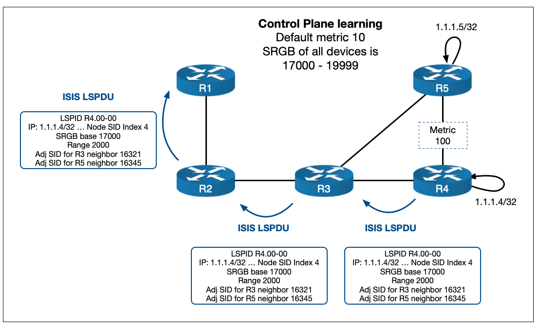
Looking at the LSPDU in the diagram above R4 is advertising….
- The 1.1.1.4/32 Prefix
- An Index of 4
- An SRGB Base of 17000
- A Range of 2000
- An unprotected IPv4 Adj-SID for each of its neighbors (R3 and R5) – other Adj-SIDs have been left out for simplicity
Now let’s consider how R2 installs entries into its LFIB for 1.1.1.4/32. R2’s best path to reach 1.1.1.4/32 is via R3 so it takes the information from both R4s LSPDU and R3s LDSPU…
In Label
R2’s In label for 1.1.1.4/32 is 17000 (its own SRGB Base) plus 4 (the Index from R4.00-00) = 17004.
Out Label
R2’s Out label for 1.1.1.4/32 is 17000 (R3’s SRGB Base which it would have got from R3.00-00) plus 4 (the Index from R4.00-00) = 17004.
You can very quickly see that if every device in the network has 17000-18999 as its SRGB, then the label will remain the same as traffic is forwarded through the network, because the In and Out labels will be the same!
From here we can illustrate how SR is a source routing paradigm. Let us assume that in our test network traffic comes into R1 and is destined for R5. However for some reason, we have a desire to send traffic over the R4-R5 link even though it is not the best IGP path. R1 can do this by stacking instructions (in the form of labels) onto the packet that other routers can interpret.
Here’s how it works:
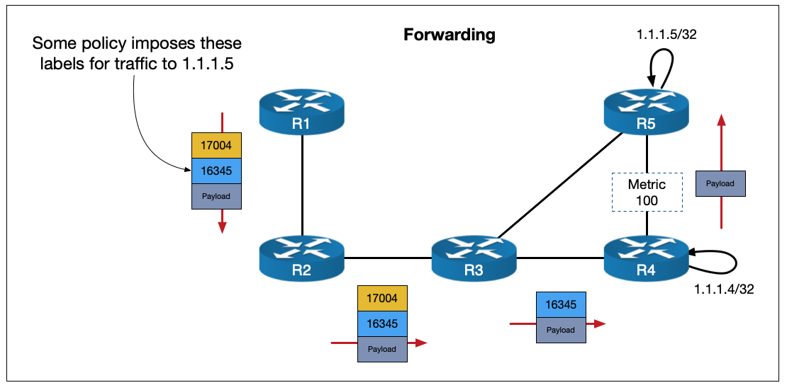
R1 has added {17004} as the top label and {16345} as the bottom of stack label. Don’t worry about how the label stack derived. There are multiple policies and protocols that can facilitate this – but that is another blog in and of itself!
If you follow the packet through the network you can see that R2 is essentially doing a swap operation to the same label. R3 is then performing standard PHP before forwarding the packet to R4 (PHP works slightly differently in Segment Routing – I won’t detail it here but for our scenario it operates the same as in LDP). R4 sees the instruction of {16345} which tells it to pop the label and send it out of the interface for its adjacency to R5 (regardless of its best path).
This illustrates a number of advantages for SR:
• The source router is doing the steering.
• There is no need to keep state. In a traditional IGP+LDP network this kind of steering is typically achieved using MPLS TE and involves RSVP signalling to the head end router and back. With SR the source simply instantiates the label stack and forwards the packet.
• No need to run LDP. You’ve now one less protocol to run and no more LDP/IGP Sync issues.
• IPv6 label forwarding: IPv6 LDP never really took off. Cisco IOS-XR routers are able to advertise node-SIDs for both IPv4 and IPv6 prefixes. This can eliminate the need for technologies like 6PE.
Before moving on I’ll briefly show how, for example, SR on R4 would be configured for IOS-XR:
segment-routing
 global-block 17000 23999 <<< the SRGB Base and range are auto calculated based on this
!
interface Loopback0
 ipv4 address 1.1.1.4 255.255.255.255
!
router isis LAB
 is-type level-2-only
 net 49.0100.1111.1111.0004.00
 address-family ipv4 unicast
  metric-style wide
  segment-routing mpls sr-prefer <<< sr-prefer is needed if LDP is also running
 !
 address-family ipv6 unicast
  metric-style wide
  segment-routing mpls sr-prefer
 !
 interface Loopback0
  passive
  address-family ipv4 unicast
   prefix-sid absolute 17004 <<< configured as absolute values but broken up in the TLV
  !
 !
 interface GigabitEthernet0/0/0/0
  point-to-point
  address-family ipv4 unicast
  !
 interface GigabitEthernet0/0/0/1
  point-to-point
  address-family ipv4 unicast
  !
 !
!
There are more types of SIDs and many more applications for Segment Routing than I have shown here – but if you’re new to SR, this brief summary should be enough to help you understand TI-LFA. With that said, let’s look at how LFA and its different flavours work…
LFA Introduction
Loop Free Alternate is a Fast Reroute (FRR) technology that basically prepares a backup path ahead of a network failure. In the event of a failure, the traffic can be forwarded into the backup path immediately (the typical goal is sub 50ms) with minimal downtime. It can be thought of as roughly analogous to EIGRPs feasible successor.
The best way to learn is by example. So what I’ll do is walk through Classic-LFA, Remote-LFA and TI-LFA showing how each improves on the last. First, however, I’ll introduce some terminology before we get to the actual topologies:
• PLR (Point of Local Repair) – The router doing the protection. This is the router that will watch for outages on its protected elements and initiate FRR behaviour if needed.
• Release Point – The point in the network where, with respect to the destination prefix, the failure of the Protect Element makes no difference. It’s the job of the PLR to get traffic to the Release Point.
• C, Protected Element – The part of the network being protected against failure. LFA can provide Link Protection, Node Protection or SRLG (Shared Risk Link Group) protection. This post only covers Link Protection, but the principle is the same.
• D, Destination prefix – LFA is done with respect to a destination. So when presenting formulas and diagrams, D, will refer to the destination prefix.
• N, Neighbor – A neighbor connected to the PLR that (in the case of Classic-LFA) is a possible Release Point for an FRR solution.
• Post-convergence path – Refers to the best path to the destination, after the network has converged around the failure.
If a failure occurs at a given PLR router, it does the following:
- Assumes that the rest of the network is NOT aware of the failure yet – i.e. all the other routers think the link is still up and their CEF entries reflect that.
- Asks itself where it can send traffic such that it will not loop back or try cross the Protected Element that just went down – or to put it another way, where is the Release Point?
- If it has a directly connected Neighbor that satisfies the previous point, then send it to that Neighbor. Nice and easy, job done. This is Classic-LFA.
- If, however, the Release Point is not directly connected, traffic will need to be tunnelled to it somehow – this is R-LFA and TI-LFA.
Now that we’ve introduced the basic mechanism, let’s start with Classic-LFA.
Classic-LFA
Here is our starting topology:
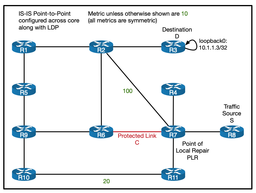
The link we’re looking to protect is the link between R6 and R7. The prefix we will be protecting is the loopback of R3 (10.1.1.3/32). Traffic will be coming from R8. This makes R7 the PLR. We haven’t implemented SR yet so we’re just working with a standard IGP + LDP model.
Download the Classic-LFA configs here.
So, if you are protecting a single link Classic-LFA (also called local-LFA) can help. The rule for Classic-LFA is this (where Dist(x,y) is the IGP cost from x to y before the failure):
Dist(N, D) < Dist (PLR, N) + Dist (PLR, D)
If the cost for the Neighbor to reach the Destination is less than the cost of the PLR to reach the Neighbor plus the cost of the PLR to get to the Destination, the Neighbor is a valid Release Point. In short, this means that traffic won’t loop back or try to use the Protected Element.
Here’s the idea using our topology:
Prior to the failure traffic takes the R8-R7-R6-R2-R3 path.
When the R6-R7 link fails R7 must figure out where to send the traffic.
It can’t send it to R11. Remember R11 isn’t aware of the outage yet and it’s best path to R3 is back via R7 so it will simply loop it back. Or to put this in the formula:
Dist(N, D) < Dist (PLR, N) + Dist (PLR, D)
Dist(R11, R3) < Dist (R7, R11) + Dist (R7, R3)
40 < 10 + 30 FALSE!
But it can send it to R2! R2’s best path to R3’s loopback doesn’t cross the R6-R7 link:
Dist(N, D) < Dist (PLR, N) + Dist (PLR, D)
Dist(R2, R3) < Dist (R7, R2) + Dist (R7, R3)
10 < 100 + 30 TRUE!
So R2 is the valid Release Point and if R6-R7 fails R7 can forward traffic immediately over to R2.
Configuration and Verification of Classic-LFA
The below IOS-XR config shows the basic IS-IS config from R7’s point of view (I’ve left out the config for IPv6 for brevity, but all attached configs and the downloadable lab contain IPv6).
! Standard traceroute showing normal traffic flow
RP/0/RP0/CPU0:R8#traceroute 10.1.1.3 source loopback 0
Wed Jul 21 18:56:04.316 UTC

Type escape sequence to abort.
Tracing the route to 10.1.1.3

 1  10.7.8.7 [MPLS: Label 16723 Exp 0] 64 msec  48 msec  53 msec
 2  10.6.7.6 [MPLS: Label 16619 Exp 0] 50 msec  52 msec  52 msec
 3  10.2.6.2 [MPLS: Label 16212 Exp 0] 56 msec  52 msec  52 msec
 4  10.2.3.3 52 msec  *  51 msec

RP/0/RP0/CPU0:R8#

! Configuration
hostname R7
!
router isis LAB
 is-type level-2-only
 net 49.0100.1111.1111.0007.00
 log adjacency changes
 address-family ipv4 unicast
  metric-style wide
  advertise passive-only
  mpls ldp auto-config
 !
 interface Loopback0
  passive
  address-family ipv4 unicast
  !
 !
 ! This is the link to R6
 interface GigabitEthernet0/0/0/1
  point-to-point
  address-family ipv4 unicast
   fast-reroute per-prefix level 2 << enable Classic LFA
   mpls ldp sync
  !
 !
<other interfaces omitted for brevity>


! Verifying LFA path via link to R2 with overall metric of 110
P/0/RP0/CPU0:R7#show isis fast-reroute 10.1.1.3/32
Wed Jul 21 18:56:24.064 UTC

L2 10.1.1.3/32 [30/115]
     via 10.6.7.6, GigabitEthernet0/0/0/1, R6, Weight: 0
       Backup path: LFA, via 10.2.7.2, GigabitEthernet0/0/0/4, R2, Weight: 0, Metric: 110
RP/0/RP0/CPU0:R7#


RP/0/RP0/CPU0:R7#show cef 10.1.1.3/32
Wed Jul 21 18:56:40.664 UTC
10.1.1.3/32, version 314, internal 0x1000001 0x0 (ptr 0xe1bd080) [1], 0x0 (0xe380928), 0xa28 (0xeddf9f0)
 Updated Jul 21 18:55:44.495
 remote adjacency to GigabitEthernet0/0/0/1
 Prefix Len 32, traffic index 0, precedence n/a, priority 3
   via 10.2.7.2/32, GigabitEthernet0/0/0/4, 5 dependencies, weight 0, class 0, backup (Local-LFA) [flags 0x300]
    path-idx 0 NHID 0x0 [0xecbd890 0x0]
    next hop 10.2.7.2/32
    remote adjacency
     local label 16723      labels imposed {16212} << R2's label for R3
   via 10.6.7.6/32, GigabitEthernet0/0/0/1, 5 dependencies, weight 0, class 0, protected [flags 0x400]
    path-idx 1 bkup-idx 0 NHID 0x0 [0xed68270 0x0]
    next hop 10.6.7.6/32
     local label 16723      labels imposed {16619}
RP/0/RP0/CPU0:R7#


RP/0/RP0/CPU0:R7#sh ip route 10.1.1.3/32
Wed Jul 21 18:56:52.408 UTC

Routing entry for 10.1.1.3/32
  Known via "isis LAB", distance 115, metric 30, type level-2
  Installed Jul 21 18:55:44.473 for 00:01:08
  Routing Descriptor Blocks
    10.2.7.2, from 10.1.1.3, via GigabitEthernet0/0/0/4, Backup (Local-LFA) << Classic-LFA
      Route metric is 110
    10.6.7.6, from 10.1.1.3, via GigabitEthernet0/0/0/1, Protected
      Route metric is 30
  No advertising protos.
RP/0/RP0/CPU0:R7#
Shortcomings of Classic-LFA
There are two common shortcomings with Classic-LFA:
• The backup path is sub-optimal. The cost for R7 to reach R3 is now R7-R2-R3 = 110. It would be more efficient to go R7-R11-R10-R9-R6-R2-R3 = 70. This is indeed the Post Convergence Path shown in the diagram above.
• Coverage is not 100%. If the link to R2 was not present, there would be no Classic-LFA backup path, since nothing satisfies the formula. If there’s no directly connected neighbor that satisfied the formula, nothing can be done!
Remote-LFA can help with some of these problems. To demonstrate this let’s remove the R2-R7 link…
Remote-LFA
Our topology now looks like this:
You can see there is no Classic-LFA path here if link C goes down. But there obviously is a backup path (namely R11-R10-R9-R6-R2-R3), but if all we had was Classic-LFA we’d have to wait for the IGP to coverage, which in most networks is too long. R-LFA can step in and help but in order to explain how it does so, we first need to define a couple of terms to describe the network from the point of view of the PLR. P and Q space…
P and Q Space
The P-space and the Q-space are a collection of nodes within the network that have a specific relationship to the PLR or Destination, with respect to the Protected Element. This sounds complicated but I’ll walk through it. P and Q don’t stand for anything – they’re just arbitrary letters. Let’s start with the P-space…
P-space: In our context, the definition of P-space is “The set of nodes such that, the shortest-path from the PLR to them does not cross the Protected Element.”
This basically represents the set of devices such that R7’s best path to them, doesn’t cross the R6-R7 link.
So to figure this out…
Start at R7 and for every other router in the network figure out R7’s best path to reach it.
Does its best path cross the R6-R7 link? (this includes all ECMP paths too!)
• yes? – then it is not the in the P-space
• no? – this it is in the P-space
In our network the P-space contains these routers:
Note that even though R7 could reach R10 via R11 with a total cost of 30, it also has an ECMP cost 30 path via R9-R6-R7, which disqualifies it.
So that’s the P-space, but what about the Q-space…?
Q-space: The formal definition of Q-space is “the set of nodes such that their shortest-path to the Destination does not cross the Protected Element.”
This basically represents the set of devices that can get to R3 (the Destination) without worrying about whether or not the R6-R7 link has failed. They are basically on the other side of the failure with respect to the Destination – or in other words, they are candidate Release Points.
So to figure this out…
Go to each router in the network and figure out its best path to reach R3.
Does its best path cross the R6-R7 link? (again, this includes all ECMP paths too!)
• yes? – then it is not in the Q-space
• no? – this it is in the Q-space
So in our network the Q-space contains these routers:

What we want is a place where P and Q overlap. If we can get it to that router we can avoid the downed Protected Element and get the traffic to the Destination.
But in our setup they don’t overlap!
However, we can use something called the extended P-space to increase our reach. So what is the extended P-space?
Think about the network from R7s point of view. R7 can’t control what other routers do once it sends a packet on its way. But it can decide which of its interfaces it sends the packet out of. This allows us to consider not just our own P-space, but also the P-space of any directly connected Neighbors that exist in our own P-space. Adding all these together forms what we call the extended P-space.
In short, the extended-P space from the point of view of any node (in our case R7), is its own P-space + the P-space of all of its directly connected P-space Neighbors.
So for R7, we calculate the P-space for R4, R11 and R8 (we don’t calculate the P-space of R6, since R6 is not in R7’s P-space).
The P-space for R4 and R8 are identical:
The P-space of R11 is a little bigger:
Again, to reiterate how we calculate R11’s P-space, look at each device in the network and include it if R11’s best path to reach it doesn’t cross C.
If we combine these, we get our extended P-space:
Now if we combine the extended P-space and the Q-space we have an overlap at R10!
Any nodes in the overlap are called PQ nodes – these will be valid Release Points. If there is more than one, R7 will select the nearest. But how do we get the traffic there? If the R6-R7 link failed and the PLR simply sent traffic to R11 it would send it straight back (remember R11 isn’t aware of the failure yet). Here’s where R-LFA and its tunnelling kick in…
Remote-LFA Tunnelling
Download the R-LFA configs here.
Once the PQ node is found, the PLR will prepare a backup path whereby it puts the protected traffic in an LSP that ends on the PQ node. This is done by pushing a label on top of the stack.
But before it does that it must do the regular LDP swap operation for the original LSP to the Destination (R3). Under normal LDP conditions, it would swap the incoming label with the local label of its downstream neighbor (learned via LDP). But in this case the R7 doesn’t have an LDP session to the PQ node (R10)… so it builds a targeted one!
Over this targeted LDP session the PQ node will tell the PLR what its local label is for the destination prefix. It is this label that the PLR will swap the transport label for before it pushes on the label that will forward traffic to the PQ node.
To put this in diagram form for our example:

In our example, R10 tells R7 what its local LDP label is for R3 loopbacks. R7 swaps the transport label for this tLDP-learned label and then pushes R11’s label for R10 on top and forwards it to R11.
All of these tLDP sessions and calculations are done ahead of time. So that switching to the backup tunnel is as fast as possible.
Configuration and Verification for R-LFA
Here’s the IOS-XR configuration and verification output for R-LFA:
! Configuration
hostname R7
!
router isis LAB
 is-type level-2-only
 net 49.0100.1111.1111.0007.00
 log adjacency changes
 address-family ipv4 unicast
  metric-style wide
  advertise passive-only
  mpls ldp auto-config
 !
 interface Loopback0
  passive
  address-family ipv4 unicast
  !
 !
 interface GigabitEthernet0/0/0/0
  point-to-point
  address-family ipv4 unicast
   fast-reroute per-prefix level 2
   fast-reroute per-prefix remote-lfa tunnel mpls-ldp << Enable R-LFA
   mpls ldp sync
  !
 <other interfaces left out for brevity>


! Verification of backup path
RP/0/RP0/CPU0:R7#show cef 10.1.1.3/32 detail
Wed Jul 21 19:07:22.598 UTC
10.1.1.3/32, version 387, internal 0x1000001 0x0 (ptr 0xe1bd080) [1], 0x0 (0xe380928), 0xa28 (0xeddfac8)
 Updated Jul 21 19:05:46.659
 remote adjacency to GigabitEthernet0/0/0/1
 Prefix Len 32, traffic index 0, precedence n/a, priority 3
  gateway array (0xe1e7da8) reference count 15, flags 0x500068, source lsd (5), 1 backups
                [6 type 5 flags 0x8401 (0xe525560) ext 0x0 (0x0)]
  LW-LDI[type=5, refc=3, ptr=0xe380928, sh-ldi=0xe525560]
  gateway array update type-time 1 Jul 21 19:04:24.215
 LDI Update time Jul 21 19:04:24.215
 LW-LDI-TS Jul 21 19:04:38.931
   via 10.7.11.11/32, GigabitEthernet0/0/0/3, 5 dependencies, weight 0, class 0, backup [flags 0x300]
    path-idx 0 NHID 0x0 [0xecbd410 0x0]
    next hop 10.7.11.11/32
    remote adjacency
     local label 16723      labels imposed {24112 24017} << 24112 is R11's label for R10 and 24017 is R10's label for R3
   via 10.6.7.6/32, GigabitEthernet0/0/0/1, 5 dependencies, weight 0, class 0, protected [flags 0x400]
    path-idx 1 bkup-idx 0 NHID 0x0 [0xed686d0 0x0]
    next hop 10.6.7.6/32
     local label 16723      labels imposed {16619}


    Load distribution: 0 (refcount 6)

    Hash  OK  Interface                 Address
    0     Y   GigabitEthernet0/0/0/1    remote
RP/0/RP0/CPU0:R7#

! Verification of R10s tLDP session and config
RP/0/RP0/CPU0:R10#sh mpls ldp neighbor 10.1.1.7:0

Peer LDP Identifier: 10.1.1.7:0
  TCP connection: 10.1.1.7:646 - 10.1.1.10:44079
  Graceful Restart: No
  Session Holdtime: 180 sec
  State: Oper; Msgs sent/rcvd: 18/18; Downstream-Unsolicited
  Up time: 00:03:58
  LDP Discovery Sources:
    IPv4: (1)
      Targeted Hello (10.1.1.10 -> 10.1.1.7, passive)
    IPv6: (0)
  Addresses bound to this peer:
    IPv4: (5)
      10.1.1.7       10.4.7.7       10.6.7.7       10.7.8.7
      10.7.11.7
    IPv6: (0)

RP/0/RP0/CPU0:R10#sh run mpls ldp
mpls ldp
 address-family ipv4
  discovery targeted-hello accept << this is needed to accept targeted LDP sessions
 !
!
RP/0/RP0/CPU0:R10#
So that’s R-LFA. It can help to reach a Release Point if it isn’t a directly connected neighbor. It’s also worth noting that R-LFA can use SR labels if they are available, rather than using tLDP.
Shortcomings of R-LFA
But there are shortcomings with R-LFA too:
• There is increased complexity with all of the tLDP sessions running everywhere.
• The backup path still might not be post-convergence path – meaning that traffic will be forwarding in a suboptimal manner while the network converges and then will need to switch to the new best path once convergence is complete.
• Coverage is still not 100% – there might not be a PQ overlap!
We’ll look at just such a case with no PQ overlap next…
TI-LFA and SR
First off, lets assume that we have removed LDP from the our network and configured SR instead. I won’t go through the process of turning LDP off and turning SR on beyond briefly showing this configuration:
segment-routing
 global-block 17000 23999 << define the SRGB
!
router isis LAB
 address-family ipv4 unicast
  no mpls ldp auto-config << turn off LDP
  metric-style wide
  segment-routing mpls sr-prefer << enable SR
 !
 interface Loopback0
  address-family ipv4 unicast
   prefix-sid absolute 17001 << statically create the node SID
  !
 !
 interface GigabitEthernet0/0/0/0
  point-to-point
  address-family ipv4 unicast
   no mpls ldp sync << turn off LDP-IGP sync
 !
!
The downloadable lab for this blog has both SR and LDP configured but SR is preferred.
Now we’ll make another change to our topology by increasing the R9-R10 metric as follows:
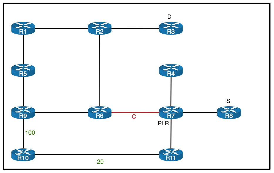
This is a subtle change. But if we go through the process of calculating the P and Q spaces we get the following:
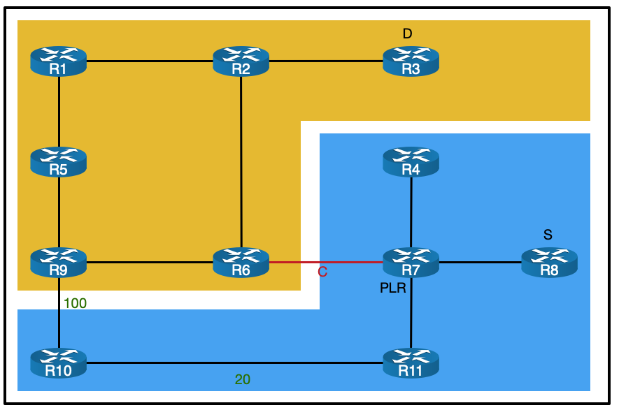
You can see there is no PQ overlap (this includes R7’s extended P-space). Let’s try to fix this using R-LFA…
We can’t do what we did last time and use R10 as the node to build our tLDP session to. If we tunnel traffic to R10, what label to we put at the bottom of the stack?
If we use R10’s local label for R3 it will forward the traffic straight back to R11 trying to use the R7-R6 link. This is precisely what it means to not be in the Q-space! It’s worth noting here that since we’re now using SR, R10’s local label for R3 with be the globally recognised 17003 label – but the problem will be the same either way, since R10s best path to R3 crosses the R7-R6 link.
Ok but what about R9…? If we try to tunnel traffic to R9, R7 will have to send traffic traffic to R11 with a top label of R11’s local label for R9 (again an SR label, namely 17009). But what will R11 do when it get’s this packet? It will send the traffic straight back to R7 (again trying to use the R7-R6 link) – if this wasn’t the case, R11 would be in the Q-space!
So what do we do? Well, here’s where the power of Segment Routing steps in. Topology Independent Loop Free Alternate (or TI-LFA) utilizes Adj-SIDs to bridge the P–Q space gap . Remember Adj-SIDs are locally generated labels communicated via the IGP TLVs that act as instructions to forward traffic to their local neighbors.
R7 does the following:
• Calculates what the best path to R3 would be if the link from R6-R7 were to go down (or in other words, it calculates the post-convergence path) – in this case it sees the best path is R7-R11-R10-R9-R6-R2-R3.
• Calculates the Segment List needed to forward traffic along this path – assuming other nodes in the network will not yet be aware of the R6-R7 failure.
• Installs this Segment List as the backup path.
The details of the algorithm used to calculate the Segment List is not publicised by Cisco, but in our case, the general principle is straight forward to grasp.
The top most label (or segment) gets the traffic to the border P node – R10.
The next label is the Adj-SID that R10 has for R9. It basically instructs R10 to pop the Adj-SID label and forward it out of its Adjacency to R9 – this is the P–Q bridging in action.
The bottom of stack label is simply the Node-SID for R3. When R9 gets it, we know it will forward it on to R3 without crossing the protected link, because it is in the Q-space.
To put this in diagram form, we get the following:

Once TI-LFA is enabled all of this is calculated and installed automatically. A key thing to highlight here is that the backup path is the same as the post-convergence path. This means that traffic will not have to change its path through the network again when the IGP converges. The only thing that will change is the label stack.
Configuration and Verification of TI-LFA
TI-LFA is pretty easy to configure and verification is straight forward when you know what to look for…
! Configuration
hostname R7
!
router isis LAB
 is-type level-2-only
 net 49.0100.1111.1111.0007.00
 log adjacency changes
 address-family ipv4 unicast
  metric-style wide
  advertise passive-only
  mpls ldp auto-config
 !
 interface Loopback0
  passive
  address-family ipv4 unicast
  !
 !
 interface GigabitEthernet0/0/0/0
  point-to-point
  address-family ipv4 unicast
   fast-reroute per-prefix level 2
   fast-reroute per-prefix ti-lfa level 2 << Enable TI-LFA
  !
 <other interfaces left out for brevity>

! Verification
RP/0/RP0/CPU0:R7#show isis fast-reroute 10.1.1.3/32 detail
Thu Jul 22 21:30:52.232 UTC

L2 10.1.1.3/32 [30/115] Label: 17003, medium priority
     via 10.6.7.6, GigabitEthernet0/0/0/1, Label: 17003, R6, SRGB Base: 17000, Weight: 0
       Backup path: TI-LFA (link), via 10.7.11.11, GigabitEthernet0/0/0/3 R11, SRGB Base: 17000, Weight: 0, Metric: 160
         P node: R10.00 [10.1.1.10], Label: 17010 <<< P and Q nodes are specified
         Q node: R9.00 [10.1.1.9], Label: 24001 <<< 24001 is R10s Adj-SID for R9
         Prefix label: 17003
         Backup-src: R3.00
       P: No, TM: 160, LC: No, NP: No, D: No, SRLG: Yes
     src R3.00-00, 10.1.1.3, prefix-SID index ImpNull, R:0 N:1 P:0 E:0 V:0 L:0,
         Alg:0
RP/0/RP0/CPU0:R7#

RP/0/RP0/CPU0:R7#show cef 10.1.1.3/32 detail
Thu Jul 22 21:31:05.178 UTC
10.1.1.3/32, version 837, labeled SR, internal 0x1000001 0x83 (ptr 0xe1ba878) [1], 0x0 (0xe3800e8), 0xa28 (0xee59a38)
 Updated May 23 15:22:46.988
 remote adjacency to GigabitEthernet0/0/0/1
 Prefix Len 32, traffic index 0, precedence n/a, priority 1
  gateway array (0xe1e7838) reference count 15, flags 0x500068, source rib (7), 1 backups
                [6 type 5 flags 0x8401 (0xe524e10) ext 0x0 (0x0)]
  LW-LDI[type=5, refc=3, ptr=0xe3800e8, sh-ldi=0xe524e10]
  gateway array update type-time 1 May 23 15:22:46.989
 LDI Update time Jul 22 20:51:34.950
 LW-LDI-TS Jul 22 20:51:34.951
   via 10.7.11.11/32, GigabitEthernet0/0/0/3, 12 dependencies, weight 0, class 0, backup (TI-LFA) [flags 0xb00]
    path-idx 0 NHID 0x0 [0xecbd770 0x0]
    next hop 10.7.11.11/32, Repair Node(s): 10.1.1.10, 10.1.1.9 << PQ nodes called repair nodes
    remote adjacency
     local label 17003      labels imposed {17010 24001 17003}
   via 10.6.7.6/32, GigabitEthernet0/0/0/1, 12 dependencies, weight 0, class 0, protected [flags 0x400]
    path-idx 1 bkup-idx 0 NHID 0x0 [0xf082510 0x0]
    next hop 10.6.7.6/32
     local label 17003      labels imposed {17003}


    Load distribution: 0 (refcount 6)

    Hash  OK  Interface                 Address
    0     Y   GigabitEthernet0/0/0/1    remote
RP/0/RP0/CPU0:R7#
Demonstration
To close off this blog I’ll give a packet capture demonstration of TI-LFA in action. In my EVE-NG lab environment, if I set a constant ping from R8 to R3 before shutting down the R6-R7 link, the IGP actually converges too fast for me capture any TI-LFA encapsulated packets. The fix this problem I updated the PLR as follows:
RP/0/RP0/CPU0:R7#conf t
Fri Aug 27 17:00:09.741 UTC
RP/0/RP0/CPU0:R7(config)#ipv4 unnumbered mpls traffic-eng Loopback0
RP/0/RP0/CPU0:R7(config)#!
RP/0/RP0/CPU0:R7(config)#mpls traffic-eng
RP/0/RP0/CPU0:R7(config-mpls-te)#!
RP/0/RP0/CPU0:R7(config-mpls-te)#router isis LAB
RP/0/RP0/CPU0:R7(config-isis)# address-family ipv4 unicast
RP/0/RP0/CPU0:R7(config-isis-af)#  microloop avoidance segment-routing
RP/0/RP0/CPU0:R7(config-isis-af)#  microloop avoidance rib-update-delay 10000
RP/0/RP0/CPU0:R7(config-isis-af)#commit
I’m not going to go into detail on what microloop avoidance is here. But put briefly a microloop is, as the name suggests, is very short term routing loop caused by the fact that different routers will update their forwarding tables at different rates after a network change. Microloop avoidance is a mechanism that uses Segment Routing to detect and avoid such conditions. The main take away here though, is the rib-update-delay command. This instructs the router to hold the LFA path in the RIB for a certain period regardless of whether or not it could converge quicker. In our case we’re instructing R7 to keep forwarding traffic along the TI-LFA backup path after the R6-R7 failure for 10 seconds (10,000 milliseconds).
Once this was sorted, I started a packet capture on R11’s interface facing R7 and repeated the test…
RP/0/RP0/CPU0:R8#ping 10.1.1.3 source lo0 repeat 10000
Fri Aug 27 17:01:29.996 UTC
Type escape sequence to abort.
Sending 10000, 100-byte ICMP Echos to 10.1.1.3, timeout is 2 seconds:
!!!!!!!!!!!!!!!!!!!!!!!!!!!!!!!!!!!!!!!!!!!!!!!!!!!!!!!!!!!!!!!!!!!!!!
!!!!!!!!!!!!!!!!!!!!!!!!!!!!!!!!!!!!!!!!!!!!!!!!!!!!!.!!!!!!!!!!!!!!!!
!!!!!!!!!!!!!!!!!!!!!!!!!!!!!!!!!!!!!!!!!!...!!!!!!!!!!!!!!!!!!!!!!!!!
!!!!!!!!!!!!!!!!!!!!!!!!!!!!!!!!!!!!!!!!!!!!!!!!.!!!!!!!!!!!!!!!!!!!!!
!!!!!!!!!!!!!!!!!!!!!!!!!!!!!!!!!!!!!!!!!!!!!!!!!!!!.!!!!!!!!!!!!!!!!!
<output omitted>
RP/0/RP0/CPU0:R7#conf t
Fri Aug 27 17:01:50.259 UTC
RP/0/RP0/CPU0:R7(config)#interface gigabitEthernet 0/0/0/1
RP/0/RP0/CPU0:R7(config-if)#shut
RP/0/RP0/CPU0:R7(config-if)#commit
Fri Aug 27 17:01:58.731 UTC
RP/0/RP0/CPU0:R7(config-if)#If we look at the PCAP on R11 we can see the correct labels are being used on the ICMP packets.

Checking R7 before the 10 seconds are up shows a backup TI-LFA tunnel in use:
RP/0/RP0/CPU0:R7#sh isis fast-reroute tunnel
Fri Aug 27 17:02:04.210 UTC

IS-IS LAB SRTE backup tunnels

tunnel-te32770, state up, type primary-uloop
  Outgoing interface: GigabitEthernet0/0/0/3
  Next hop: 10.7.11.11
  Label stack: 17010, 24001
  Prefix: 10.1.1.1/32 10.1.1.2/32 10.1.1.3/32 10.1.1.5/32 10.1.1.6/32 10.1.1.9/32

RP/0/RP0/CPU0:R7#
The Prefix field shows all of the IGP destinations for which R7 will use this tunnel. Note that 10.1.1.3/32 is in that list. You can try this yourself in the downloadable lab.
Conclusions
So that’s TI-LFA using SR! I’ve tried to present this blog as a basic introduction to LFA types as well as a demonstration of how powerful SR can be. There are more nuanced scenarios involving a mix of SR-capable and LDP-only nodes, but LDP/SR interoperation is another topic entirely. We’ve seen how traditional technologies like Classic LFA and R-LFA are adequate in most circumstance but TI-LFA with the power of SR can provide complete coverage. Thank you for reading.
It’s not easy building GRE
The importance of having backup paths in a network isn’t a revelation to anyone. From HSRP on a humble pair of Cisco 887s to TI-LFA integration on an ASR9k, having a reliable backup path is a staple for all modern networks.
This quirk looks at the need for a backup path on a grand scale. We’ll look at a hypothetical scenario of a multi-national ISP losing a backup path to a whole region and how, as a rapid response solution, it builds a redundant path over a Transit Provider…
Scenario
So here is our hypothetical Tier 2 Service Provider network. It is spread across three cities in three different countries and has various Peering and Transit connections throughout:

IS-IS and LDP is run internally. This includes the international links, resulting in one contiguous IGP domain. What’s important to note here is that New York only has a single link to the other countries and only has one Tier 1 Transit Provider.
The quirk
To setup this quirk, we need a link failure to take place. Let’s say a deep-sea dredger rips up the cable in the Atlantic going from New York to London.

New York doesn’t lose access – it still has a link to the rest of the network via Paris. However that link to Paris is now its sole connection to the rest of the network. In other words, New York no longer has that all important backup path. The situation is exacerbated when you learn that a repair boat won’t be sent to fix the undersea cable for weeks!
So what do you do?
You could invest in more fibre and undersea cabling to connect your infrastructure – arguably you should’ve already done this! But placing an order for a Layer 2 Service or contacting a Tier 1 Provider to setup CsC takes time. By all means, place the order. But in the meantime, you’ll need to set something up quickly in case New York to Paris fails and New York becomes completely isolated.
One option, and indeed the one we’ll explore in this blog, is to reconnect New York to London through your transit provider without waiting for an order or even involving them at all…
I should preface this by stating that this solution is neither scalable nor sustainable. But it is most definitely an interesting and … well… quirky work around that can be deployed at a pinch.
With that said, how do we actually do this?
In order to connect New York to London over another network, we’ll need to implement tunnelling of some kind. Specifically, we’ll look at creating a GRE tunnel between the MSEs in New York and London using the Tier 1 Transit Provider as the underlay network.
To put it in diagram form, our goal is to have something like this:

To guide us through this setup, I’ll tackle the process step by step using the following sections:
- Tunnel-end point Reachability
- Control Plane: The IPs of endpoints of the GRE tunnel will need reachability over the Tier 1 Transit Provider.
- Data Plane: Traffic between the endpoint must be able to flow. This section will examine what packet filtering might need adjusting.
- GRE tunnel configuration
- Control Plane: This covers the configuration and signalling of the GRE tunnel
- Data Plane: We’ll need to look at MTU and account for the additional overhead added by the GRE headers.
- Tunnel overlay protocols: Making sure IS-IS and LDP can be run over the GRE tunnel, including the proper transport addresses and metrics.
- Link Capacity: This new tunnel will need to be able to take the same amount of traffic that typically flows to and from New York. Given that our control over this is limited, we’ll assume that there is sufficient bandwidth on these links.
- RTBH: Any Remote Trigger Black Holing mechanisms that have been applied to your Transit ports may need to have exceptions made so it does not mistake your own traffic for a DDoS attack.
- Security: You could optionally encrypt the traffic transiting the Transit Providers network.
The goal of this quirk is to explore the routing and reachability side of the scenario so I will discuss the first 3 of the above points in detail and assume that link capacity, RTBH and security are already accounted for.
Downloadable Lab
This quirk considers the point of view of a large Service Provider with potentially hundreds of routers. However in order to demonstrate the configuration specifics and allow you to try the setup, I’ve built a small scale lab to emulate the solution. I’ve altered some of the output shown in this blog to make it appear more realistic. As such, the lab and output shown in this post don’t match each other verbatim. But I’ll turn to the lab towards the end in order to do a couple of traceroutes and for the most part the IP addressing and configuration match enough for you to follow along.
I built the lab in EVE-NG so it can be download as a zipped UNL file. I’ve also provided a zip file containing the configuration for each node, in case you’re using a different lab emulation program.

With that said, let’s take a look at how we’d set this up…
Tunnel-end point Reachability – Control Plane
We’ll start by putting some IP addressing on the topology:
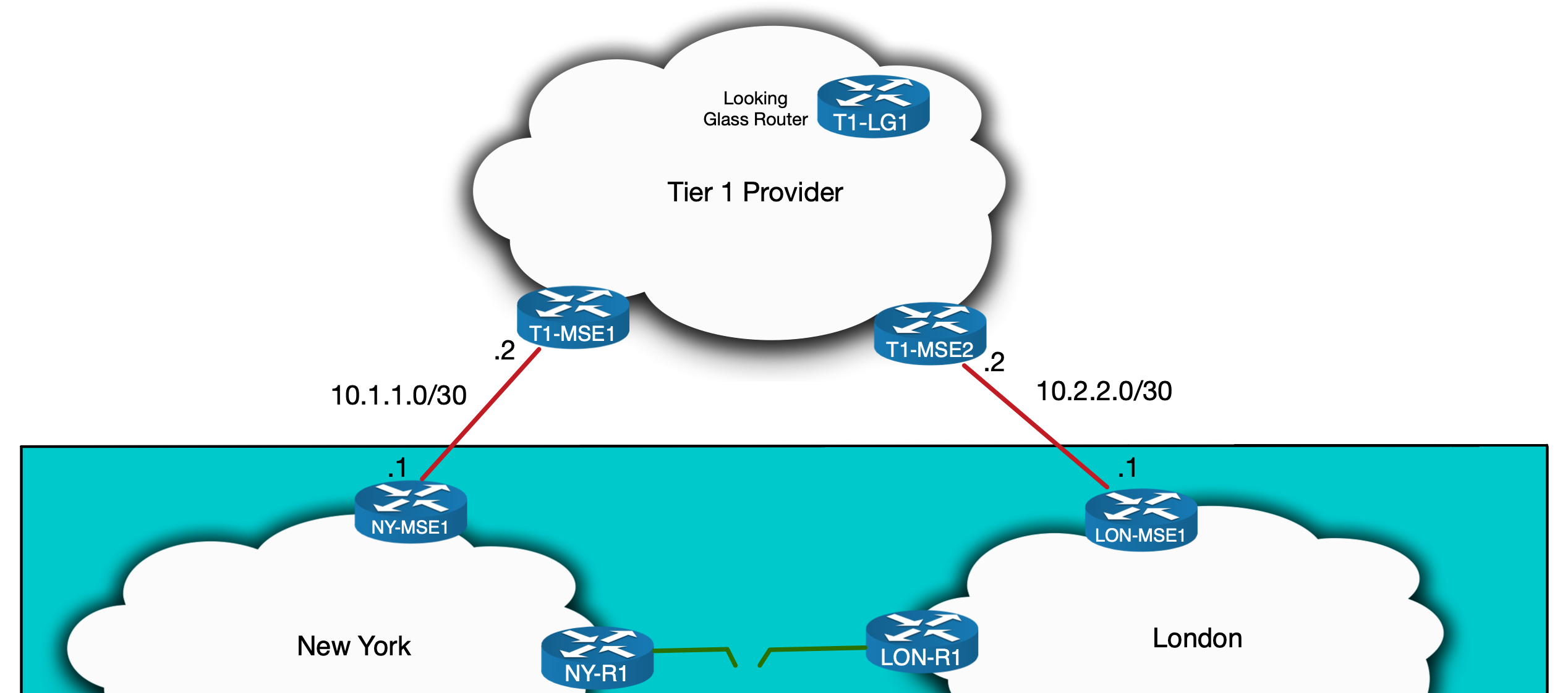
(the addressing used throughout will be private, but in a real world scenario it would be public)
Now we might first try to build the tunnel directly between our routers, using 10.1.1.1 and 10.2.2.1 as the respective endpoints. But if we try to ping and trace from one to the other we see it fails:
RP/0/RSP0/CPU0:NY-MSE1#show route ipv4 10.2.2.1
Routing entry for 10.2.0.0/16
  Known via "bgp 500", distance 20, metric 0
  Tag 100, type external
  Installed Jul 12 15:36:41.110 for 2w2d
  Routing Descriptor Blocks
    10.1.1.2, from 10.1.1.2, BGP external
      Route metric is 0
  No advertising protos.
RP/0/RSP0/CPU0:NY-MSE1#ping 10.2.2.1
Wed Jul 26 15:26:21.374 EST
Type escape sequence to abort.
Sending 5, 100-byte ICMP Echos to 10.2.2.1, timeout is 2 seconds:
.....
Success rate is 0 percent (0/5)
RP/0/RSP0/CPU0:NY-MSE1#traceroute 10.2.2.1

Type escape sequence to abort.
Tracing the route to 10.2.2.1

 1  10.1.1.2 2 msec  1 msec  1 msec
 2  10.117.23.3 [MPLS: Label 43567 Exp 0] 34 msec  35 msec  35 msec
 3  10.117.23.17 [MPLS: Label 34234 Exp 0] 35 msec  36 msec  35 msec
 4  10.117.23.57 [MPLS: Label 94571 Exp 0] 36 msec  46 msec  35 msec
 5  10.117.23.23 [MPLS: Label 64066 Exp 0] 35 msec  35 msec  35 msec
 6   *  *  *
 7   *  *  *
 8   *  *  *
 9   *  *  *
RP/0/RSP0/CPU0:NY-MSE1#
From the traceroute we can see that traffic is entering an LSP in the Tier 1 MPLS core. The IPs we see are likely the loopback addresses of the P routers along the path. In spite of this limited visibility we can see the traffic isn’t reaching its destination – it is stopping at 10.117.23.23. But why?
Well, we don’t have full visibility of the Tier 1 Provider’s network, but they are likely restricting access to the transport subnets used to connect to their downstream customers. This is a common practice and is designed to, among other things, prevent customers from having access to networks that their Tier 1 edge devices exist on. Traffic should never go to these transport addresses, they should only go through them.
This means that when we see the traceroute stop at 10.117.23.23, this may very well be an ACL or filter on T1-MSE2 blocking traffic to 10.2.2.0/30 from an unauthorised source.

As a result of this, we’ll have to advertise a subnet to the Tier1 Provider from each side and have them act as the tunnel endpoints. Tier1 Providers typically don’t accept any prefix advertisement smaller than a /24 so in this case we’ll have no choice but to sacrifice two such ranges – one for each site. See why I mentioned this is not scalable?
Before we allocate these ranges, I’m going to assume the following points have already been fulfilled:
- The /24 address ranges are available and unused: let’s say we have a well documented IPAM (IP Address Management) system and can find a couple of /24s.
- The Transit Provider will accept the prefixes we advertise – meaning our RIR records are up to date and any RPKI ROAs are correctly configured so that the Transit Provider will not have any problems accepting the /24s advertised over BGP.
With these assumptions in place, we’ll start by allocating a subnet for each site (again, pretend these are public):
- New York subnet: 172.16.10.0/24
- London subnet: 172.16.20.0/24
At this point we need to see what the Transit Provider sees in order to make sure our routes are being received correctly. For this we’ll use a Looking Glass. To illustrate this, I’ve invented a hypothetical Transit Provider called TEAR1 Limited (a bad pun I know, but fit for our purposes 😛 ). I’ve put together images demonstrating what a Looking Glass website for TEAR1 might look like. First, we’ll specify that we want to find BGP routing information about 172.16.10.0:

After clicking submit, we might get a response similar to what you see below:

So what can we make out from the above output…? We can see, for example, that T1-LG1 is receiving the prefix from what looks like a Route Reflector (evident by the existence of a Cluster List in the BGP output) and from what is probably the T1-MSE1 Edge Router that receives the prefix from our ISP. The path to the Edge Router is being preferred, since it has a Cluster List length of zero. T1-LG1 could itself be a Reflector within TEAR1. It’s difficult to tell much more without knowing the full internal topology of TEAR1, but the main take home here is that is it sees a /16, rather than the more specific /24s. This is fine at this point – we haven’t configured anything yet. And indeed if we check NY-MSE1 we can see that we are originating a /16 as part of our normal prefix advertisements to Transit Providers:
RP/0/RSP0/CPU0:NY-MSE1#show route ipv4 172.16.0.0/16

Routing entry for 172.16.0.0/16
  Known via "static", distance 1, metric 0 (connected)
  Installed May 26 12:53:27.539 for 8w1d
  Routing Descriptor Blocks
    directly connected, via Null0
      Route metric is 0, Wt is 1
  No advertising protos.
RP/0/RSP0/CPU0:NY-MSE1#sh bgp ipv4 uni neigh 10.1.1.2 adv | in 172.16.0.0
172.16.0.0/16     10.1.1.1   Local           500i
RP/0/RSP0/CPU0:NY-MSE1#
Here we’re using a null route for the subnet. This is common within Service Providers. The null route is redistributed into BGP and advertised to TEAR1. This isn’t a problem since within our Service Provider there will be plenty of subnets with the 172.16.0.0/16 supernet – meaning there will always be more specific routes to follow. We could have alternatively used BGP aggregation.
Regardless of how this is done, we need to configure NY-MSE1 to advertise 172.16.10.0/24 to TEAR1 and LON-MSE1 to advertise 172.16.20.0/24. We could use static null routes here too, but remember the goal is to have these IPs be the endpoints of the GRE tunnel. With this in mind, we’ll use loopbacks and advertise them into BGP using the network statement. The overall configuration is as follows:
! (NY-MSE1)
interface Loopback10
 description Temporary GRE end-point
 ipv4 address 172.16.10.1 255.255.255.0
!
router bgp 500
 address-family ipv4 unicast
  network 172.16.10.0/24
(I’ve only shown the config for the New York side but the London side is analogous – obviously replacing 172.16.10.0 with 172.16.20.0. To save showing duplicate output, I will sometimes only show the New York side, but know that in those cases, the equivalent substituted config is on the London side.)
To advertise these ranges to TEAR1 we’ll need to adjust our outbound BGP policies.
I’ll pause here to note that filtering on both the control plane and data planes at a Service Provider edge is a complex subject. The CLI I’ve shown here is grossly oversimplified just to demonstrate the parts relevant to this quirk (including a couple of hypothetical communities that could be used for various routing policies). The ACL and route policies in a real network will be more complicated and cover more aspects of routing security, including anti-spoofing and BGP hi-jack prevention. That being said, here is the config we need to apply:
! (NY-MSE1)
router bgp 500
  address-family ipv4 unicast
   network 172.16.10.0/24
  !
 neighbor 10.1.1.2
  remote-as 100
  description TEAR1-BGP-PEER
  address-family ipv4 unicast
   send-community-ebgp
   route-policy TEAR1-OUT in
   route-policy TEAR1-IN in
   remove-private-AS
  !
!
route-policy TEAR1-OUT
  if community matches-any NO-TRANSIT then
    drop
  elseif community matches-any NEW-YORK-ORIGIN and destination in OUR-PREFIXES then
    pass
  elseif destination in (172.16.10.0/24) then
    set community (no-export)
    pass
  else
    drop
  endif
end-policy
And indeed if we soft clear the BGP sessions and check the Looking Glass again, we can see that TEAR1 now sees both /24 subnets.
RP/0/RSP0/CPU0:NY-MSE1#clear bgp ipv4 unicast 10.1.1.2 soft
RP/0/RSP0/CPU0:NY-MSE1#sh bgp ipv4 uni neigh 10.1.1.2 adv | include 172.16.10.0
172.16.10.0/24     10.1.1.1   Local           500i
RP/0/RSP0/CPU0:NY-MSE1#

RP/0/RSP0/CPU0:LON-MSE1#clear bgp ipv4 unicast 10.2.2.2 soft
RP/0/RSP0/CPU0:LON-MSE1#sh bgp ipv4 uni neigh 10.2.2.2 adv | include 172.16.20.0
172.16.20.0/24     10.2.2.1   Local           500i
RP/0/RSP0/CPU0:LON-MSE1#
You might’ve noticed in the above output the inclusion of the no-export community. This is done to make sure that TEAR1 does not advertise these /24s to any of its fellow Tier 1 Providers and pollute the internet further. By “polluting the internet” I mean introducing unnecessary prefixes into the global internet routing table. In this case, we are adding two /24s which, from the point of view of the rest of the internet, aren’t needed since we’re already advertising the /16. We can’t make TEAR1 honour the no-export community, but it is a reasonable precaution to put in place nonetheless.
This covers control plane advertisements to TEAR1. But we also need to think about how LON-MSE1 sees NY-MSE1s loopback and vice versa. Each MSE should see the GRE tunnel endpoint of the other over the TEAR1 connection. Depending on how we perform redistribution, we might see these tunnel endpoints in iBGP or in our IGP. But we don’t want them to see each over our own core or else that is the path the tunnel will take!
In addition to this, we don’t want TEAR1 to advertise our own IP addresses back to us. Most ISPs filter against this anyways, and even if we didn’t, BGP loop-prevention (seeing our own ASN in the AS_PATH attribute) would prevent our MSEs from accepting them.
The cleanest way to ensure NY-MSE1 has a best path for 172.16.20.0 via TEAR1 (and vice versa) is a static route:
! NY-MSE1
router static
 address-family ipv4 unicast
  172.16.20.1/32 TenGigE0/0/0/1 10.1.1.2 description GRE_Tunnel

! LON-MSE1
router static
 address-family ipv4 unicast
  172.16.10.1/32 TenGigE0/0/0/1 10.2.2.2 description GRE_Tunnel

RP/0/RSP0/CPU0:NY-MSE1#sh ip ro 172.16.20.1

Routing entry for 172.16.20.1/32
  Known via "static", distance 1, metric 0
  Installed Jul 7 18:34:18.727 for 1w2d
  Routing Descriptor Blocks
    10.1.1.2, via TenGigE0/0/0/1
      Route metric is 0, Wt is 1
  No advertising protos.
RP/0/RSP0/CPU0:NY-MSE1#
This will make sure that the tunnel is built over the Transit Provider. The data plane needs to be adjusted next, to allow the actual traffic to flow…
Tunnel-end point Reachability – Data Plane
Many Service Providers will apply inbound filters on Peering and Transit ports both on the control plane and data plane. This is done to, among other things, prevent IP spoofing. For example, any outbound traffic should have a source address that is part of the Service Providers address space (or from the PI Space of any of it customers). Similarly, any inbound traffic should have a source address that is not part of their customer address space. These are the types of things we’ll need to consider when opening up the data plane for our GRE tunnel.
For this scenario, let’s assume we block inbound traffic that is sourced from our own address space. This would prevent spoofed traffic crossing our network, but it would also block traffic from one of our GRE tunnel endpoints to the other. We’ll need to adjust the inbound ACL and to make this as secure as possible we should only allowing GRE traffic from and to the relevant /32 endpoints.
I’ve omitted the full details of this ACL, since in real life it would be too long to show. However here is the addition we’d need to make (assuming no reject statements before index 10):
! NY-MSE1
interface TenGigE0/0/0/1
 description Link to T1-MSE1
 ipv4 address 10.1.1.1 255.255.255.252
 ipv4 access-group FROM-TRANSIT ingress
!
ipv4 access-list IN-FROM-TRANSIT
 <<output omitted>>
 10 permit gre host 172.16.20.1 host 172.16.10.1
 <<output omitted>>
!
We’re now in a position to test connectivity – remembering to source from loopback10 so that LON-MSE1 has a return route:
RP/0/RSP0/CPU0:NY-MSE1#traceroute 10.2.2.1 source loopback 10

Type escape sequence to abort.
Tracing the route to 172.16.20.1

 1  10.1.1.2 2 msec  1 msec  1 msec
 2  10.117.23.3 [MPLS: Label 43567 Exp 0] 34 msec  35 msec  35 msec
 3  10.117.23.17 [MPLS: Label 34234 Exp 0] 35 msec  36 msec  35 msec
 4  10.117.23.57 [MPLS: Label 94571 Exp 0] 36 msec  46 msec  35 msec
 5  10.117.23.23 [MPLS: Label 64066 Exp 0] 35 msec  35 msec  35 msec
 6  10.2.2.1 msec *  60 msec
RP/0/RSP0/CPU0:NY-MSE1#
Success, it works! We have loopback to loopback reachability across TEAR1 and we didn’t even need to give them so much as a phone call. To put this in diagram format, here is where we are at:

We’re now ready to configure the GRE tunnel.
Configuring the Tunnel – Control Plane
The GRE configuration itself is fairly straight forward. We’ll configure the tunnel endpoint on each router, specifying the loopbacks as the sources. We also need to allocate IPs on the tunnel interfaces themselves. These will form an internal point-to-point subnet that will be used to establish the IS-IS and LDP neighborships we need. Let’s allocate 192.168.1.0/30, with NY-MSE1 being .1 and LON-MSE1 being .2.
The config looks like this:
! NY-MSE1
interface tunnel-ip100
 ipv4 address 192.168.1.1/30
 tunnel mode gre ipv4
 tunnel source Loopback10
 tunnel destination 172.16.20.1
!

! LON-MSE1
interface tunnel-ip100
 ipv4 address 192.168.1.2/30
 tunnel mode gre ipv4
 tunnel source Loopback10
 tunnel destination 172.16.10.1
!
Checking the GRE tunnel shows that it is up:
RP/0/RSP0/CPU0:NY-MSE1#sh interface tunnel-ip 100 detail
tunnel-ip100 is up, line protocol is up
  Interface state transitions: 3
  Hardware is Tunnel
  Internet address is 192.168.1.1/30
  MTU 1500 bytes, BW 100 Kbit (Max: 100 Kbit)
     reliability 255/255, txload 2/255, rxload 2/255
  Encapsulation TUNNEL_IP,  loopback not set,
  Last link flapped 1w2d
  Tunnel TOS 0
  Tunnel mode GRE IPV4
  Keepalive is disabled.
  Tunnel source 172.16.10.1(Loopback100), destination 172.16.20.1/32
  Tunnel TTL 255
  Last input 00:00:00, output 00:00:00
  Last clearing of "show interface" counters never
  5 minute input rate 1000 bits/sec, 1 packets/sec
  5 minute output rate 1000 bits/sec, 1 packets/sec
     264128771 packets input, 58048460659 bytes, 34 total input drops
     0 drops for unrecognized upper-level protocol
     Received 0 broadcast packets, 0 multicast packet
     115204515 packets output, 72846125759 bytes, 0 total output drops
     Output 0 broadcast packets, 0 multicast packets
RP/0/RSP0/CPU0:NY-MSE1#sh interface tunnel-ip 100 brief

               Intf       Intf        LineP              Encap  MTU        BW
               Name       State       State               Type (byte)    (Kbps)
--------------------------------------------------------------------------------
              ti100          up          up          TUNNEL_IP  1500        100


RP/0/RSP0/CPU0:LON-MSE1#sh interfaces tunnel-ip100 detail
tunnel-ip100 is up, line protocol is up
  Interface state transitions: 5
  Hardware is Tunnel
  Internet address is 192.168.1.2/30
  MTU 1500 bytes, BW 100 Kbit (Max: 100 Kbit)
     reliability 255/255, txload 2/255, rxload 2/255
  Encapsulation TUNNEL_IP,  loopback not set,
  Last link flapped 1w2d
  Tunnel TOS 0
  Tunnel mode GRE IPV4
  Keepalive is disabled.
  Tunnel source 172.16.20.1 (Loopback100), destination 172.16.10.1/32
  Tunnel TTL 255
  Last input 00:00:00, output 00:00:00
  Last clearing of "show interface" counters never
  5 minute input rate 1000 bits/sec, 1 packets/sec
  5 minute output rate 1000 bits/sec, 1 packets/sec
     115176196 packets input, 73259625130 bytes, 0 total input drops
     0 drops for unrecognized upper-level protocol
     Received 0 broadcast packets, 0 multicast packets
     264158130 packets output, 57031343960 bytes, 0 total output drops
     Output 0 broadcast packets, 0 multicast packets
RP/0/RSP0/CPU0:LON-MSE1#
So now we have the GRE tunnel up and running. Before we look at the MTU changes, I want to demonstrate how the MTU issue manifests itself by configuring the overlay protocols first…
Tunnel overlay protocols – LDP
The LDP configuration is, on the face of it, quite simple.
! Both LON-MSE1 and NY-MSE1
mpls ldp
 interface tunnel-ip100
  address-family ipv4
  !
 !
!
This will actually cause the session to come up, however on closer inspection the setup is not a typical one. (in this output NY-MSE and LON-MSE have loopback0 addresses of 2.2.2.2/32 and 22.22.22.22/32 respectively).
RP/0/0/CPU0:NY-MSE1#sh mpls ldp discovery
Thu Jul 23 19:52:06.959 UTC

Local LDP Identifier: 2.2.2.2:0
Discovery Sources:
  Interfaces:

    <<output to core router omitted>>

    tunnel-ip100 : xmit/recv
      VRF: 'default' (0x60000000)
      LDP Id: 22.22.22.22:0, Transport address: 22.22.22.22
          Hold time: 15 sec (local:15 sec, peer:15 sec)
          Established: Jul 23 19:50:14.967 (00:01:52 ago)

RP/0/0/CPU0:NY-MSE1#sh mpls ldp neighbor
Thu Jul 23 19:54:21.940 UTC

    <<output to core router omitted>>

Peer LDP Identifier: 22.22.22.22:0
  TCP connection: 22.22.22.22:54279 - 2.2.2.2:646
  Graceful Restart: No
  Session Holdtime: 180 sec
  State: Oper; Msgs sent/rcvd: 25/25; Downstream-Unsolicited
  Up time: 00:02:30
  LDP Discovery Sources:
    IPv4: (1)
      tunnel-ip100
    IPv6: (0)
  Addresses bound to this peer:
    IPv4: (5)
      10.2.2.1       10.20.24.2     22.22.22.22    172.16.20.1
      192.168.1.2
    IPv6: (0)

RP/0/0/CPU0:NY-MSE1#
To explain the above output it’s worth quickly reviewing LDP (see here for a cheat sheet). LDPs Hellos, with a TTL of 1 are sent to 224.0.0.2 (the all routers multicast address) out of all interfaces with LDP enabled. This includes the GRE tunnel. This means that LON-MSE1 and NY-MSE1 establish an Hello Adjacency over the tunnel. Once this Adjacency is up, the router with the lower LDP Router ID will establish a TCP Session to the transport address of the other (from its own transport address). The transport address is included in the LDP Hellos. This address defaults to the LDP Router ID which in turn defaults to the highest numbered loopback. This allocation of the Router ID only occurs once (on IOS-XR) when LDP is first initialised and from then on, only when the existing Router ID is changed. As a result, depending on the order in which loopbacks and LDP are introduced, the Router ID might not necessarily be the current highest loopback address. In the output above we can see that the TCP Session is established between the loopback0s of each router. This is the loopback used to identify the node and is used for things like the source address of iBGP sessions. What’s key here is that each routers path to the other routers loopback0 address is internal – over the IGP. This means the TCP Session is established over our own core.

This isn’t a problem initially – LDP would come up and labels would be exchanged. But if our last link to New York via Paris goes down, this will cause the TCP Session to drop. It should come back up with IS-IS configured over the GRE tunnel, but this kind of disruption, combined with delays associated with LDP-IGP synchronisation, could result in significant downtime.
The wiser option is to configure the transport addresses to the be the GRE tunnel endpoints. This will ensure the TCP Session will be established over the GRE tunnel from the start…
! NY-MSE1
mpls ldp
 address-family ipv4
 !
 interface tunnel-ip100
  address-family ipv4
   discovery transport-address 192.168.1.1
  !
 !
!

! LON-MSE1
mpls ldp
 address-family ipv4
 !
 interface tunnel-ip100
  address-family ipv4
   discovery transport-address 192.168.1.2
  !
 !
!
Once this is done we can see the transport address changes accordingly:
RP/0/0/CPU0:NY-MSE1#sh mpls ldp discovery
Fri Jul 24 23:30:40.832 UTC

Local LDP Identifier: 2.2.2.2:0
Discovery Sources:
  Interfaces:

    <<output to core router omitted>>

    tunnel-ip100 : xmit/recv
      VRF: 'default' (0x60000000)
      LDP Id: 22.22.22.22:0, Transport address: 192.168.1.2
          Hold time: 15 sec (local:15 sec, peer:15 sec)
          Established: Jul 24 23:29:58.135 (00:00:42 ago)

RP/0/0/CPU0:NY-MSE1#sh mpls ldp neighbor
Fri Jul 24 23:30:44.472 UTC

    <<output to core router omitted>>

Peer LDP Identifier: 22.22.22.22:0
  TCP connection: 192.168.1.2:43187 - 192.168.1.1:646
  Graceful Restart: No
  Session Holdtime: 180 sec
  State: Oper; Msgs sent/rcvd: 23/23; Downstream-Unsolicited
  Up time: 00:00:32
  LDP Discovery Sources:
    IPv4: (1)
      tunnel-ip100
    IPv6: (0)
  Addresses bound to this peer:
    IPv4: (5)
      10.2.2.1       10.20.24.2     22.22.22.22    172.16.20.1
      192.168.1.2
    IPv6: (0)

RP/0/0/CPU0:NY-MSE1#
It’s also a good idea to manually configure the LDP Router ID to ensure that transport address connectivity is not reliant on an automatic process (I found when labbing this scenario that the LDP Router ID was, at times, defaulting to loopback10 used for the GRE Tunnel. Since I was not redistributing this loopback into IS-IS, this resulted in the neighboring P router not having a route to this address to establish the TCP session. Hardcoding the LDP Router ID to loopback0s address solved this).
Now that IS-IS is up, we can move on to the IGP configuration.
Tunnel overlay protocols – IS-IS
The IS-IS configuration across the GRE tunnel is done just like any interface. The only thing to remember here is to set the metric to be high enough such that under normal circumstances traffic will go via Paris (output from here on is taken from the downloadable lab, in case you notice subtle differences from the output given so far).
RP/0/0/CPU0:NY-MSE1#conf t
Mon Jul 27 21:51:08.282 UTC
RP/0/0/CPU0:NY-MSE1(config)#router isis LAB
RP/0/0/CPU0:NY-MSE1(config-isis)# interface tunnel-ip100
RP/0/0/CPU0:NY-MSE1(config-isis-if)#  circuit-type level-2-only
RP/0/0/CPU0:NY-MSE1(config-isis-if)#  point-to-point
RP/0/0/CPU0:NY-MSE1(config-isis-if)#  address-family ipv4 unicast
RP/0/0/CPU0:NY-MSE1(config-isis-if-af)#   metric 1000
RP/0/0/CPU0:NY-MSE1(config-isis-if-af)#   mpls ldp sync
RP/0/0/CPU0:NY-MSE1(config-isis-if-af)#  !
RP/0/0/CPU0:NY-MSE1(config-isis-if-af)#commit
Mon Jul 27 21:51:18.292 UTC
RP/0/0/CPU0:Jul 27 21:51:18.541 : config[65742]: %MGBL-CONFIG-6-DB_COMMIT :
Configuration committed by user 'user1'. Use 'show configuration commit changes
1000000073' to view the changes.
RP/0/0/CPU0:NY-MSE1(config-isis-if-af)#RP/0/0/CPU0:Jul 27 21:51:28.231 :
isis[1010]: %ROUTING-ISIS-5-ADJCHANGE : Adjacency to LON-MSE1 (tunnel-ip100)
(L2) Up, New adjacency
RP/0/0/CPU0:Jul 27 21:51:28.751 : isis[1010]: %ROUTING-ISIS-4-SNPTOOBIG : L2 SNP
size 1492 too big for interface tunnel-ip100 MTU 1476, trimmed to interface MTU

RP/0/0/CPU0:NY-MSE1(config-isis-if-af)#
RP/0/0/CPU0:Jul 27 21:51:52.309 : config[65742]: %MGBL-SYS-5-CONFIG_I : Configured
from console by user1
RP/0/0/CPU0:NY-MSE1#show isis neighbor
Mon Jul 27 21:51:57.699 UTC

IS-IS LAB neighbors:
System Id      Interface        SNPA           State Holdtime Type IETF-NSF
P1             Gi0/0/0/2        *PtoP*         Up    24       L2   Capable
LON-MSE1       ti100            *PtoP*         Up    20       L2   Capable

Total neighbor count: 2
RP/0/0/CPU0:NY-MSE1#
Once IS-IS comes up, you might notice the following log message:
RP/0/0/CPU0:Jul 27 21:54:23.419 : isis[1010]: %ROUTING-ISIS-4-SNPTOOBIG : L2
SNP size 1492 too big for interface tunnel-ip100 MTU 1476, trimmed to interface MTU
This leads us to the last topic we need to explore, MTU…
MTU
To consider MTU, let’s first see what the MTU currently is:
RP/0/0/CPU0:NY-MSE1#show interface GigabitEthernet 0/0/0/1
Mon Jul 27 22:04:12.558 UTC
GigabitEthernet0/0/0/1 is up, line protocol is up
  Interface state transitions: 1
  Hardware is GigabitEthernet, address is 5000.000c.0002 (bia 5000.000c.0002)
  Internet address is 10.1.1.1/30
  MTU 1514 bytes, BW 1000000 Kbit (Max: 1000000 Kbit)
     reliability 255/255, txload 0/255, rxload 0/255
  Encapsulation ARPA,
  Full-duplex, 1000Mb/s, unknown, link type is force-up
  <<output omitted>>
In IOS-XR the 14 bytes of the Layer 2 header needs to be accounted for (6 bytes for Source MAC + 6 bytes for Destination MAC + 2 Bytes for the Ethertype) so the 1514 bytes in the above output equates to a Layer 3 MTU of 1500.
If we look at the GRE tunnel MTU it too shows 1500 and unlike the physical interface MTU it doesn’t need account for the layer 2 header.
RP/0/0/CPU0:NY-MSE1#show interface tunnel-ip100
Mon Jul 27 22:07:48.454 UTC
tunnel-ip100 is up, line protocol is up
  Interface state transitions: 1
  Hardware is Tunnel
  Internet address is 192.168.1.1/30
  MTU 1500 bytes, BW 100 Kbit (Max: 100 Kbit)
     reliability 255/255, txload 2/255, rxload 2/255
  Encapsulation TUNNEL_IP,  loopback not set,
  Last link flapped 1d00h
  Tunnel TOS 0
  Tunnel mode GRE IPV4,
  Keepalive is disabled.
  Tunnel source 172.16.10.1 (Loopback10), destination 172.16.20.1
  Tunnel TTL 255
  <<output omitted>>
But what the MTU in the above output doesn’t show is that the tunnel has to add a 24 byte GRE header, reducing the effective MTU of the link. If we use the following command we can see that the Layer 3 IPv4 MTU is 1476 (1500 -24):
RP/0/0/CPU0:NY-MSE1#show im database interface tunnel-ip100
Mon Jul 27 22:13:42.299 UTC

View: OWN - Owner, L3P - Local 3rd Party, G3P - Global 3rd Party, LDP - Local
      Data Plane
      GDP - Global Data Plane, RED - Redundancy, UL - UL

Node 0/0/CPU0 (0x0)

Interface tunnel-ip100, ifh 0x00000090 (up, 1500)
  Interface flags:          0x0000000000034457 (REPLICATED|STA_REP|TUNNEL
                            |IFINDEX|VIRTUAL|CONFIG|VIS|DATA|CONTROL)
  Encapsulation:            gre_ipip
  Interface type:           IFT_TUNNEL_GRE
  Control parent:           None
  Data parent:              None
  Views:                    UL|GDP|LDP|G3P|L3P|OWN

  Protocol        Caps (state, mtu)
  --------        -----------------
  None            gre_ipip (up, 1500)
  clns            clns (up, 1476)
  ipv4            ipv4 (up, 1476)
  mpls            mpls (up, 1476)

RP/0/0/CPU0:NY-MSE1#
This explains the IS-IS log message we were seeing:
RP/0/0/CPU0:Jul 27 21:54:23.419 : isis[1010]: %ROUTING-ISIS-4-SNPTOOBIG : L2
SNP size 1492 too big for interface tunnel-ip100 MTU 1476, trimmed to interface MTU
IS-IS is trying to send a packet that is bigger than 1476 bytes and so it must reduce the MTU size. This doesn’t have an impact on the IS-IS session in our case, but is worth noting.
To better understand the exact MTU breakdown, let’s visualise what happens when a packet arrives at NY-MSE1 headed for the GRE tunnel.
The packet arrives looking like this:
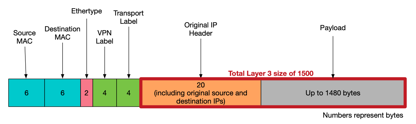
The MSE will then add the 24 bytes of GRE headers before sending it the Transit Provider, making the packet look like this:

So what is the impact of this? Will traffic be able to flow over the link?
Well in short, yes. But hosts will tend to sent packets of 1500 bytes (which includes the IP Header). With the additional Label and GRE headers in place, the packet will be fragmented as it is sent over TEAR1.
To illustrate this, I’ll turn to a pcap on EVE lab used to simulate this scenario. We’ll look at what happens if the link to Paris actual fails and our GRE tunnel is brought into action!
The lab contains a customer VRF with two sites, A and B. Loopback1 on the CE at each site is used to represent a LAN range. We can ping or trace from one site to another and watch its behaviour across the core. The lab includes a single link between the London and New York parts of the network used to represent the path via Paris. If we bring this link down, traffic will start to flow over the GRE tunnel. We can then do a pcap on NY-MSE1 to T1-MSE1 link to see the fragmentation. Here’s the setup:

First bring down our link to London:
P1(config)#int Gi4
P1(config-if)#shut
P1(config-if)#
*Jul 27 22:29:20.447: %LDP-5-NBRCHG: LDP Neighbor 44.44.44.44:0 (4) is DOWN
(Interface not operational)
*Jul 27 22:29:20.548: %CLNS-5-ADJCHANGE: ISIS: Adjacency to P2 (GigabitEthernet4)
Down, interface deleted(non-iih)
*Jul 27 22:29:20.549: %CLNS-5-ADJCHANGE: ISIS: Adjacency to P2 (GigabitEthernet4)
Down, interface deleted(non-iih)
P1(config-if)#
Then do a trace and ping while pcap’ing the outbound interface to T1-MSE1:
CE1#trace 192.168.70.1 source loopback1
Type escape sequence to abort.
Tracing the route to 192.168.70.1
VRF info: (vrf in name/id, vrf out name/id)
  1 172.30.1.9 46 msec 5 msec 1 msec
  2 10.10.14.4 [AS 500] [MPLS: Labels 1408/2107 Exp 0] 43 msec 15 msec 22 msec
  3 10.10.24.2 [AS 500] [MPLS: Labels 24003/2107 Exp 0] 46 msec 13 msec 12 msec
  4 192.168.1.2 [AS 500] [MPLS: Labels 24001/2107 Exp 0] 53 msec 15 msec 12 msec
  5 10.20.24.4 [AS 500] [MPLS: Labels 2402/2107 Exp 0] 31 msec 34 msec 13 msec
  6 172.30.1.13 [AS 500] [MPLS: Label 2107 Exp 0] 32 msec 13 msec 20 msec
  7 172.30.1.14 [AS 500] 54 msec *  44 msec
CE1#ping 192.168.70.1 source loopback 1 size 1500
Type escape sequence to abort.
Sending 5, 1500-byte ICMP Echos to 192.168.70.1, timeout is 2 seconds:
Packet sent with a source address of 192.168.60.1
!!!!!
Success rate is 100 percent (5/5), round-trip min/avg/max = 18/38/111 ms
CE1#
The PCAP shows fragmentation taking place on the ICMP packets:
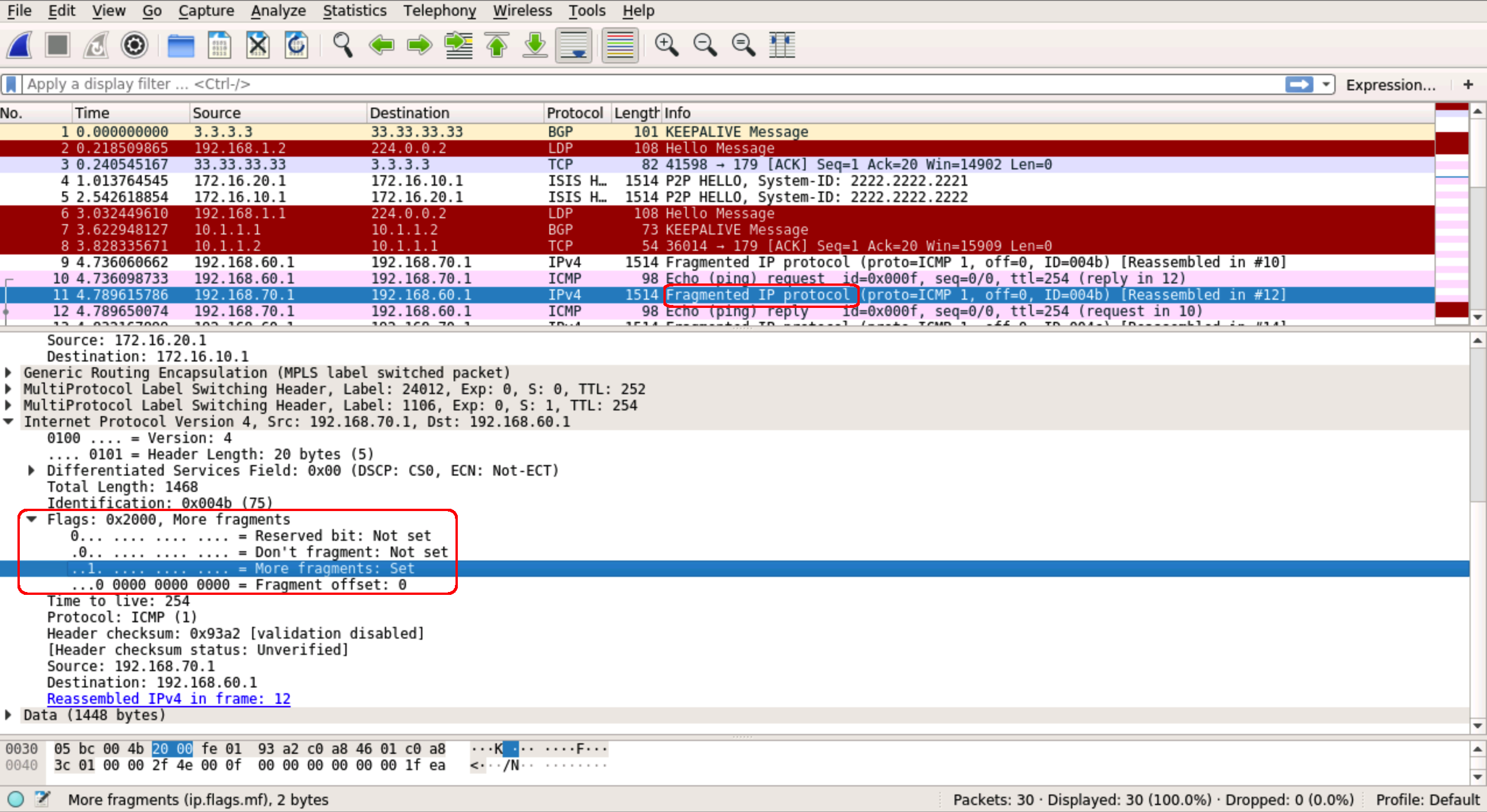
Indeed if we ping with the df bit set we see it doesn’t get through:
CE1#ping 192.168.70.1 source loopback1 size 1500 df-bit
Type escape sequence to abort.
Sending 5, 1500-byte ICMP Echos to 192.168.70.1, timeout is 2 seconds:
Packet sent with a source address of 192.168.60.1
Packet sent with the DF bit set
.....
Success rate is 0 percent (0/5)
CE1#
Fragmentation should generally be avoided where possible. To that end, we’ll need to adjust the MTU to allow our end host to sent at its usual 1500 bytes without fragmentation.
We will need to add 32 bytes to the already 1514 MTU. The breakdown is as follows:
- Original IP Header and Data – 1500
- VPN Label – 4
- Transport Label – 4
- GRE Header – 24
- Layer 2 Headers – 14
- TOTAL: 1546
So of we set the MTU to 1546 we’ll be able to send a packet of 1500 bytes across our core. Remember for the GRE tunnel we don’t need bother accounting for the 14 bytes of layer 2 overhead:
RP/0/0/CPU0:NY-MSE1(config)#interface tunnel-ip100
RP/0/0/CPU0:NY-MSE1(config-if)#mtu 1532
RP/0/0/CPU0:NY-MSE1(config-if)#interface GigabitEthernet0/0/0/1
RP/0/0/CPU0:NY-MSE1(config-if)#mtu 1546
RP/0/0/CPU0:NY-MSE1(config-if)#commit

RP/0/0/CPU0:LON-MSE1(config)#interface tunnel-ip100
RP/0/0/CPU0:LON-MSE1(config-if)#mtu 1532
RP/0/0/CPU0:LON-MSE1(config-if)#interface GigabitEthernet0/0/0/1
RP/0/0/CPU0:LON-MSE1(config-if)#mtu 1546
RP/0/0/CPU0:LON-MSE1(config-if)#commit
Once this done we can see that sending exactly 1500 bytes from our customer site works:
CE1#ping 192.168.70.1 source loopback1 size 1501 df-bit
Type escape sequence to abort.
Sending 5, 1501-byte ICMP Echos to 192.168.70.1, timeout is 2 seconds:
Packet sent with a source address of 192.168.60.1
Packet sent with the DF bit set
.....
Success rate is 0 percent (0/5)
CE1#ping 192.168.70.1 source loopback1 size 1500 df-bit
Type escape sequence to abort.
Sending 5, 1500-byte ICMP Echos to 192.168.70.1, timeout is 2 seconds:
Packet sent with a source address of 192.168.60.1
Packet sent with the DF bit set
!!!!!
Success rate is 100 percent (5/5), round-trip min/avg/max = 14/41/110 ms
CE1#
One final point to note here is that the Layer 3 MTU of the interface on the other end of the Transit link must be at least 1532 otherwise IS-IS will not come up across the GRE tunnel. This is unfortunately something that, as the Tier 2 Provider, we don’t control. In fact, any MTU along the part of the path that we don’t control could result in fragmentation. The best we can do in this case is to configure it and see. If IS-IS isn’t up after the MTU changes, we would have to revert and simply put up with the fragmentation.
So that’s it! An interesting solution to a somewhat rare and bespoke problem. Hopefully this blog has provided some insight into how Service Providers operate and how various technologies interrelate with one another to reach an end goal of maintaining redundancy. Again, I stress that this solution is not scalable, but I think it’s an entertaining look into what can be accomplished if you think outside the box. Feel free to download the lab and have a play around. Maybe you can see a different way to approach the scenario? Thoughts and feedback are welcome as always.
Routing loop shambles
Hey everyone! It’s been a while since I posted anything, but I’ve come across this interesting quirk in my studies which I think would be of interest for anyone studying OSPF, BGP and how they work together. Comments and thoughts are welcome as always.
This blog introduces the concept of OSPF sham-links and how they can be used to influence OSPF routes across an MPLS core. It also explores how, if not used carefully, routing loops could occur with disastrous effects.
As a reminder, once I’ve set up the scenario, I’ll go through the quirk (explaining the problem), the search (finding a solution) and the work (implementing the solution) as usual.
Scenario
This scenario looks at a standard MPLS customer with two sites. These sites use OSPF as the PE-CE routing protocol and have a backdoor link between them over which OSPF is run – joining both sites into area 0.
The diagram looks like this:

I’ve labbed this in GNS3 and all routers are IOS-XE devices except for XR1 and XR2 which, as the names suggest, are IOS-XR boxes.
LAN ranges have been simulated using loopbacks. Each PE is doing redistribution from OSPF into MP-BGP (internal, external 1 and external 2) and from MP-BGP into OSPF.
The design goal here is to have both sites connected in OSPF area 0 using the backdoor link as a backup – with traffic normally preferring to go over the MPLS network (or OSPF super backbone). XR1 and R1 should back each other up. Only if both of these are down should traffic traverse the backdoor link.
I’ll first introduce the problems inherent in the default behaviour as shown in the diagram above – focusing on how R4 and R5 would reach LAN1 (192.168.70.0/24) on R7. I’ll then go into how a sham-link can help solve these problems. However, as we will see in the quirk, if sham-links aren’t applied correctly some problems could appear.
OSPF and MPLS
We’ll start by looking at how OSPF and MPLS interact. For now, let’s assume the backdoor link is shutdown.
OSPF is being used between the PEs and CEs. So the PEs find themselves redistributing from OSPF into MP-BGP. When this is done, MP-BGP will set these OSPF specific community/values into the resulting VPNv4 prefix:
- The domain ID – this is an extended community taken from the process ID on the router and is considered when redistributing back into OSPF (more on that below).
- The route-type – an extended community broken up into 3 parts: the area, the LSA type and an additional option.
- The OSPF router id – another extended community representing the router sourcing this VPNv4 prefix.
- The OSPF cost is copied to the MED value.
Here we can see the output from R3 as it has redistributed the OSPF route for LAN 1 into BGP:
R3#sh run | sec router ospf
router ospf 1 vrf A
 router-id 3.3.3.3
 redistribute bgp 1 subnets
 network 10.3.7.3 0.0.0.0 area 0
R3#sh bgp vpnv4 unicast vrf A 192.168.70.0
BGP routing table entry for 1:1:192.168.70.0/24, version 77
Paths: (1 available, best #1, table A)
  Advertised to update-groups:
     1
  Refresh Epoch 1
  Local
    10.3.7.7 (via vrf A) from 0.0.0.0 (3.3.3.3)
      Origin incomplete, metric 2, localpref 100, weight 32768,
        valid, sourced, best
      Extended Community: RT:100:100
              OSPF DOMAIN ID:0x0005:0x000000010200
        OSPF RT:0.0.0.0:2:0 OSPF ROUTER ID:3.3.3.3:0
      mpls labels in/out 24/nolabel
      rx pathid: 0, tx pathid: 0x0
R3#
You can see the Domain ID field is set to 0x0005:0x000000010200. The 00000001 section represents process ID 1. MED is 2 – this represents the OSPF cost of 2 to reach LAN1. The RT is 0.0.0.0:2:0 and router-ID is 3.3.3.3:0.
NB. IOS-XR doesn’t encode the domain ID by default. For this scenario we will assume it has been configured on XR1 using the following commands:
RP/0/RP0/CPU0:XR1(config)#router ospf 1
RP/0/RP0/CPU0:XR1(config-ospf)# vrf A
RP/0/RP0/CPU0:XR1(config-ospf-vrf)# domain-id type 0005 value 000000010200
What’s important to consider here is how the PEs on the other end of the MPLS network redistribute this back into OSPF on the other side.
When the MP-BGP prefix is redistributed back into OSPF by either R1 or XR1, it uses the domain ID to determine if the route should appear as inter-area or external (I’m using colour coding here to help with differentiating between area descriptions… and because trying to read inter and intra when they occur in the same sentence makes my head hurt). If the Process ID section of the Domain ID in the VPNv4 prefix matches the local OSPF process ID on the PE doing the redistribution, then the prefix will be sent into OSPF using an inter-area Type 3 LSA. If it doesn’t, it will be an external Type 5 LSA.
In our setup, the Domain ID and Process ID all match – so when R4 and R5 receive the Type 3 LSA they see it as inter-area:
R4#sh ip route 192.168.70.0
Routing entry for 192.168.70.0/24
  Known via "ospf 1", distance 110, metric 3, type inter area
  Last update from 10.4.11.11 on GigabitEthernet1.411, 00:01:13 ago
  Routing Descriptor Blocks:
  * 10.4.11.11, from 11.11.11.11, 00:01:13 ago, via GigabitEthernet1.411
      Route metric is 3, traffic share count is 1
R4#sh ip ospf database summary 192.168.70.0

            OSPF Router with ID (4.4.4.4) (Process ID 1)

                Summary Net Link States (Area 0)

  LS age: 86
  Options: (No TOS-capability, DC, Downward)
  LS Type: Summary Links(Network)
  Link State ID: 192.168.70.0 (summary Network Number)
  Advertising Router: 1.1.1.1
  LS Seq Number: 80000001
  Checksum: 0x36CF
  Length: 28
  Network Mask: /24
        MTID: 0         Metric: 2

  LS age: 86
  Options: (No TOS-capability, DC, Downward)
  LS Type: Summary Links(Network)
  Link State ID: 192.168.70.0 (summary Network Number)
  Advertising Router: 11.11.11.11
  LS Seq Number: 80000001
  Checksum: 0x9D4
  Length: 28
  Network Mask: /24
        MTID: 0         Metric: 2

R4#
This all looks well and good. It’s worth pointing out here, that OSPF has a preference for which path to select based on the route types. The order of preference is as follows*:
- Intra-Area (O)
- Inter-Area (O IA)
- External Type 1 (E1)
- NSSA Type 1 (N1)
- External Type 2 (E2)
- NSSA Type 2 (N2)
(* This is for Cisco IOS software older than 15.1(2)S. During and after 15.1(2)S sees the E and N orders reversed. This isn’t relevant to this blog but worth noting)
It doesn’t matter what the OSPF cost is. If OSPF has the option of an intra-area route over an inter-area or external route, it will pick the intra-area option every time. Keeping that in mind, let’s bring up the backdoor link and see what happens…
The backdoor link
You might already be able to predict that as soon as we bring up the backdoor link, R4 and R5 will immediately see LAN1 as an intra-area route:
R5#conf t
Enter configuration commands, one per line.  End with CNTL/Z.
R5(config)#
%SYS-5-CONFIG_I: Configured from console by console
R5(config)#interface gi1.57
R5(config-subif)#no shut
R5(config-subif)#
%OSPF-5-ADJCHG: Process 1, Nbr 7.7.7.7 on GigabitEthernet1.57 from DOWN to INIT,
  Received Hello
%OSPF-5-ADJCHG: Process 1, Nbr 7.7.7.7 on GigabitEthernet1.57 from INIT to 2WAY,
 2-Way Received
%OSPF-5-ADJCHG: Process 1, Nbr 7.7.7.7 on GigabitEthernet1.57 from 2WAY to EXSTART,
 AdjOK?
R5(config-subif)#
%OSPF-5-ADJCHG: Process 1, Nbr 7.7.7.7 on GigabitEthernet1.57 from EXSTART to
 EXCHANGE, Negotiation Done
%OSPF-5-ADJCHG: Process 1, Nbr 7.7.7.7 on GigabitEthernet1.57 from EXCHANGE to
 LOADING, Exchange Done
%OSPF-5-ADJCHG: Process 1, Nbr 7.7.7.7 on GigabitEthernet1.57 from LOADING to FULL,
 Loading Done
R5(config-subif)#do sh ip route 192.168.70.0
Routing entry for 192.168.70.0/24
  Known via "ospf 1", distance 110, metric 101, type intra area
  Last update from 10.5.7.7 on GigabitEthernet1.57, 00:00:17 ago
  Routing Descriptor Blocks:
  * 10.5.7.7, from 7.7.7.7, 00:00:17 ago, via GigabitEthernet1.57
      Route metric is 101, traffic share count is 1
R5(config-subif)#
R5(config-subif)#do sh ip ospf database router 7.7.7.7

            OSPF Router with ID (5.5.5.5) (Process ID 1)

                Router Link States (Area 0)

  LS age: 37
  Options: (No TOS-capability, DC)
  LS Type: Router Links
  Link State ID: 7.7.7.7
  Advertising Router: 7.7.7.7
  LS Seq Number: 800000C1
  Checksum: 0x840E
  Length: 60
  AS Boundary Router
  Number of Links: 3

    Link connected to: a Stub Network
     (Link ID) Network/subnet number: 192.168.70.0
     (Link Data) Network Mask: 255.255.255.0
      Number of MTID metrics: 0
       TOS 0 Metrics: 1

    Link connected to: a Transit Network
     (Link ID) Designated Router address: 10.5.7.7
     (Link Data) Router Interface address: 10.5.7.7
      Number of MTID metrics: 0
       TOS 0 Metrics: 100

    Link connected to: a Transit Network
     (Link ID) Designated Router address: 10.3.7.7
     (Link Data) Router Interface address: 10.3.7.7
      Number of MTID metrics: 0
       TOS 0 Metrics: 1

R5(config-subif)#
You may also have spotted that the previous Type 3 LSA is no longer present. This is because the PE routers that were doing the redistribution from MP-BGP now prefer the local OSPF path. MP-BGP (iBGP from the reflectors in this case) has an administrative distance of 200. OSPF has an administrative distance of 110. OSPF wins and since redistribution takes place from the RIB, there are no MP-BGP routes to redistribute into OSPF:
R4#sh ip ospf database summary 192.168.70.0

            OSPF Router with ID (4.4.4.4) (Process ID 1)
R4#
R1#sh ip route vrf A 192.168.70.0

Routing Table: A
Routing entry for 192.168.70.0/24
  Known via "ospf 1", distance 110, metric 102, type intra area
  Redistributing via bgp 1
  Advertised by bgp 1 match internal external 1 & 2
  Last update from 10.1.5.5 on GigabitEthernet1.15, 00:04:30 ago
  Routing Descriptor Blocks:
  * 10.1.5.5, from 7.7.7.7, 00:04:30 ago, via GigabitEthernet1.15
      Route metric is 102, traffic share count is 1
R1#
Now you might be asking why I bothered to outline the difference between the PE redistributing the BGP prefix as inter-area versus external, if the R4 and R5 are just going to pick the intra-area route regardless. Well this becomes relevant when we consider how we are going to make the MPLS core the preferred path to reach LAN1.
As it stands at the moment, no matter how high we set the metric on the link between R5 and R7, traffic from Site 2 to LAN1 will always go over the backdoor link. In short, we need a way to make an intra-area route appear over the MPLS core. Here’s were sham-links come in.
Sham-Links
A sham-link is similar to an OSPF Virtual-Link but it can be run as any area and is designed for just these types of scenarios. Essentially, the PEs at either end establish an OSPF neighborship and consider themselves to be directly connected within the same area. This will all allow Type 1 and Type 2 LSAs to appear over MPLS – simulating a point-to-point connection between PEs. Let’s look at how this is setup…
Each PE creates a new loopback and puts it into vrf A. The sham-link is configured between these loopbacks.
Here’s the diagram and config for the setup:

R3#conf t
Enter configuration commands, one per line.  End with CNTL/Z.
R3(config)#interface Loopback33
R3(config-if)#vrf forwarding A
R3(config-if)#ip address 33.3.3.3 255.255.255.255
R3(config-if)#exit
R3(config)#router ospf 1 vrf A
R3(config-router)#area 0 sham-link 33.3.3.3 111.11.11.11
R3(config-router)#exit
R3(config)#router bgp 1
R3(config-router)#address-family ipv4 vrf A
R3(config-router-af)#network 33.3.3.3 mask 255.255.255.255
RP/0/RP0/CPU0:XR1#conf
RP/0/RP0/CPU0:XR1(config)#interface Loopback111
RP/0/RP0/CPU0:XR1(config-if)#vrf A
RP/0/RP0/CPU0:XR1(config-if)#ipv4 address 111.11.11.11/32
RP/0/RP0/CPU0:XR1(config-if)#root
RP/0/RP0/CPU0:XR1(config)#router ospf 1
RP/0/RP0/CPU0:XR1(config-ospf)#vrf A
RP/0/RP0/CPU0:XR1(config-ospf-vrf)#address-family ipv4 unicast
RP/0/RP0/CPU0:XR1(config-ospf-vrf)#area 0
RP/0/RP0/CPU0:XR1(config-ospf-vrf-ar)#sham-link 111.11.11.11 33.3.3.3
RP/0/RP0/CPU0:XR1(config-ospf-vrf-ar)#root
RP/0/RP0/CPU0:XR1(config)#router bgp 1
RP/0/RP0/CPU0:XR1(config-bgp)#vrf A
RP/0/RP0/CPU0:XR1(config-bgp-vrf)#rd 1:1
RP/0/RP0/CPU0:XR1(config-bgp-vrf)#address-family ipv4 unicast
RP/0/RP0/CPU0:XR1(config-bgp-vrf-af)#network 111.11.11.11/32Now it’s important to pause there and highlight a key requirement: We need to make sure that each PE has reachability to the others sham-link loopback over MPLS but not over OSPF. To that end, we should not enable OSPF on the PEs new loopbacks.
But why is this?
To answer this, consider how R3 learns about 111.11.11.11/32. If XR1 were to enable OSPF on this loopback, it would include it as a connected network in its Type 1 LSA. This would be then be communicated throughout the OSPF area, across the backdoor link and arrive at R3. All devices are in the same area so their view of the LSDB would be the same. Assuming loopback111 is also redistributed into BGP, R3 would now have two options to reach it – one via OSPF with administrative distance or 110 and one via iBGP with an administrative distance of 200.

OSPF would naturally win and the sham-link would be built over the backdoor link, which defeats the very goal we are trying to achieve! As such, we have to make sure that OSPF is not enabled on loopback 111 or loopback 33.
But, I hear you ask, what if we are still redistributing from MP-BGP into OSPF? Won’t R3 still see the path to loopback 111 via an external Type 5 LSA, which will still have a lower AD than iBGP’s 200?
Well, yes, but OSPF has a loop prevention mechanism built into it to prevent just such a thing…
When an LSA is created from redistributing from MP-BGP to OSPF, an OSPF feature called the down-bit is set in the resulting LSA. The down-bit ensures that any prefixes that are redistributed from MP-BGP into OSPF are not then redistributed back into MP-BGP. So whist R3 will see the Type 5 LSA in its LSDB it will not consider it as a valid route since it is already getting the prefix via MP-BGP and the down-bit indicates that it came from MP-BGP.

Here is the LSA as seen in the LSDB.
R5#sh ip ospf database external 111.11.11.11

            OSPF Router with ID (5.5.5.5) (Process ID 1)

                Type-5 AS External Link States

  LS age: 881
  Options: (No TOS-capability, DC, Downward)
  LS Type: AS External Link
  Link State ID: 111.11.11.11 (External Network Number )
  Advertising Router: 1.1.1.1
  LS Seq Number: 8000004D
  Checksum: 0x245C
  Length: 36
  Network Mask: /32
        Metric Type: 2 (Larger than any link state path)
        MTID: 0
        Metric: 1
        Forward Address: 0.0.0.0
        External Route Tag: 3489660929

  LS age: 1998
  Options: (No TOS-capability, DC, Downward)
  LS Type: AS External Link
  Link State ID: 111.11.11.11 (External Network Number )
  Advertising Router: 3.3.3.3
  LS Seq Number: 80000055
  Checksum: 0xD798
  Length: 36
  Network Mask: /32
        Metric Type: 2 (Larger than any link state path)
        MTID: 0
        Metric: 1
        Forward Address: 0.0.0.0
        External Route Tag: 3489660929

R5#
And if we check, we find that R3’s best path is via MP-BGP.
R3#sh ip route vrf A 111.11.11.11

Routing Table: A
Routing entry for 111.11.11.11/32
  Known via "bgp 1", distance 200, metric 0, type internal
  Redistributing via ospf 1
  Advertised by ospf 1 subnets
  Last update from 11.11.11.11 19:34:53 ago
  Routing Descriptor Blocks:
  * 11.11.11.11 (default), from 2.2.2.2, 19:34:53 ago
      Route metric is 0, traffic share count is 1
      AS Hops 0
      MPLS label: 24018
      MPLS Flags: MPLS Required
R3#
This loop prevention mechanism isn’t crucial to understanding the operation of the sham-link but it will come into play later on when we look at a potential routing loop.
Getting back to the sham-link, once we configure everything as outlined above the link comes up:
RP/0/RP0/CPU0:XR1#sh ospf vrf A sham-links

Sham Links for OSPF 1, VRF A

Sham Link OSPF_SL0 to address 33.3.3.3 is up
Area 0, source address 111.11.11.11
IfIndex = 1
  Run as demand circuit
  DoNotAge LSA allowed., Cost of using 1
  Transmit Delay is 1 sec, State POINT_TO_POINT,
  Timer intervals configured, Hello 10, Dead 40, Wait 40, Retransmit 5
    Hello due in 00:00:06:794
    Adjacency State FULL (Hello suppressed)
    Number of DBD retrans during last exchange 0
    Index 2/2, retransmission queue length 0, number of retransmission 0
    First 0(0)/0(0) Next 0(0)/0(0)
    Last retransmission scan length is 0, maximum is 0
    Last retransmission scan time is 0 msec, maximum is 0 msec
RP/0/RP0/CPU0:XR1#sh ospf vrf A neighbor

* Indicates MADJ interface
# Indicates Neighbor awaiting BFD session up

Neighbors for OSPF 1, VRF A

Neighbor ID     Pri   State           Dead Time   Address         Interface
3.3.3.3         1     FULL/  -           -        33.3.3.3        OSPF_SL0
    Neighbor is up for 00:01:20
4.4.4.4         1     FULL/BDR        00:00:39    10.4.11.4       Gi0/0/0/0.411
    Neighbor is up for 19:32:22

Total neighbor count: 2
RP/0/RP0/CPU0:XR1#
R3#sh ip ospf sham-links
Sham Link OSPF_SL8 to address 111.11.11.11 is up
Area 0 source address 33.3.3.3
  Run as demand circuit
  DoNotAge LSA allowed. Cost of using 1 State POINT_TO_POINT,
  Timer intervals configured, Hello 10, Dead 40, Wait 40,
    Hello due in 00:00:07
    Adjacency State FULL (Hello suppressed)
    Index 1/2/2, retransmission queue length 0, number of retransmission 0
    First 0x0(0)/0x0(0)/0x0(0) Next 0x0(0)/0x0(0)/0x0(0)
    Last retransmission scan length is 0, maximum is 0
    Last retransmission scan time is 0 msec, maximum is 0 msec
R3#
Both routers establish an OSPF adjacency and see each other as connected over a point-to-point link:
RP/0/RP0/CPU0:XR1#sh ospf vrf A database router 11.11.11.11
Thu Oct  3 12:31:10.478 UTC

            OSPF Router with ID (11.11.11.11) (Process ID 1, VRF A)

                Router Link States (Area 0)

  LS age: 151
  Options: (No TOS-capability, DC)
  LS Type: Router Links
  Link State ID: 11.11.11.11
  Advertising Router: 11.11.11.11
  LS Seq Number: 800000ef
  Checksum: 0xc78
  Length: 48
  Area Border Router
  AS Boundary Router
   Number of Links: 2

    Link connected to: another Router (point-to-point)
     (Link ID) Neighboring Router ID: 3.3.3.3
     (Link Data) Router Interface address: 0.0.0.1
      Number of TOS metrics: 0
       TOS 0 Metrics: 1

    Link connected to: a Transit Network
     (Link ID) Designated Router address: 10.4.11.11
     (Link Data) Router Interface address: 10.4.11.11
      Number of TOS metrics: 0
       TOS 0 Metrics: 1

RP/0/RP0/CPU0:XR1#
What’s interesting here is how XR1 sees the path to LAN1 over the sham-link:
RP/0/RP0/CPU0:XR1#sh route vrf A ipv4 192.168.70.0/24
Thu Oct  3 12:31:43.212 UTC

Routing entry for 192.168.70.0/24
  Known via "bgp 1", distance 200, metric 2, type internal
  Installed Oct  3 12:28:40.433 for 00:03:04
  Routing Descriptor Blocks
    3.3.3.3, from 2.2.2.2
     Nexthop in Vrf: "default", Table: "default", IPv4 Unicast, Table Id:0xe0000000
     Route metric is 2
  No advertising protos.
RP/0/RP0/CPU0:XR1#
It sees it as a BGP route and not an OSPF route! If we look at its BGP entry we see this:
RP/0/RP0/CPU0:XR1#sh bgp vpnv4 unicast vrf A 192.168.70.0
Thu Oct  3 12:32:15.246 UTC
BGP routing table entry for 192.168.70.0/24,Route Distinguisher: 1:1
Versions:
  Process           bRIB/RIB  SendTblVer
  Speaker                462         462
Last Modified: Oct  3 12:28:40.387 for 00:03:37
Paths: (2 available, best #1)
  Not advertised to any peer
  Path #1: Received by speaker 0
  Not advertised to any peer
  Local
    3.3.3.3 (metric 20) from 2.2.2.2 (3.3.3.3)
      Received Label 24
      Origin incomplete, metric 2, localpref 100, valid, internal, best,
          group-best, import-candidate, imported
      Received Path ID 0, Local Path ID 1, version 462
      Extended community: OSPF domain-id:0x5:0x000000010200
         OSPF route-type:0:2:0x0 OSPF router-id:3.3.3.3 RT:100:100
      Originator: 3.3.3.3, Cluster list: 2.2.2.2
      Source AFI: VPNv4 Unicast, Source VRF: A, Source Route Distinguisher: 1:1
  Path #2: Received by speaker 0
  Not advertised to any peer
  Local
    3.3.3.3 (metric 20) from 12.12.12.12 (3.3.3.3)
      Received Label 24
      Origin incomplete, metric 2, localpref 100, valid, internal,
        import-candidate, imported
      Received Path ID 0, Local Path ID 0, version 0
      Extended community: OSPF domain-id:0x5:0x000000010200
         OSPF route-type:0:2:0x0 OSPF router-id:3.3.3.3 RT:100:100
      Originator: 3.3.3.3, Cluster list: 12.12.12.12
      Source AFI: VPNv4 Unicast, Source VRF: A, Source Route Distinguisher: 1:1
RP/0/RP0/CPU0:XR1#
It is clearly an OSPF based route. The OSPF attributes are all present. But how can an OSPF path over the sham-link appear as a BGP route?
Remember that in order to send traffic across the MPLS core two labels will be needed. The top label represents the next-hop PE. This will typically be repeatedly swapped as the packet crosses the core (unless we’re using segment routing but that’s a whole other story). The second and bottom label is the VPN label used to represent this customers prefix or VRF. This label is needed since the core P routers won’t know anything of the customer subnets. This label is communicated in the VPNv4 update from R3 as it redistributes LAN1 into MP-BGP.
Here is the logical process that XR1 is follows:
- XR1 runs the Dijkstra algorithm to find LAN1, taking the sham-link into account as a point-to-point link.
- If the sham-link wins, XR1 will then use a VPNv4 route for LAN1, which in this case is being redistributed by R3. The best VPNv4 route will be used and placed in the BGP RIB instead of an OSPF route.
This is logic is due to the recursion that is taking place over the sham-link:
RP/0/RP0/CPU0:XR1#show cef vrf A 192.168.70.0
Thu Oct  3 12:41:27.680 UTC
192.168.70.0/24, version 679, internal 0x5000001 0x0 (ptr 0xdf126ec) [1], 0x0
  (0xe0d88e8), 0xa08 (0xe4dc4e8)
 Updated Oct  3 12:28:40.444
 Prefix Len 24, traffic index 0, precedence n/a, priority 3
   via 3.3.3.3/32, 3 dependencies, recursive [flags 0x6000]
    path-idx 0 NHID 0x0 [0xd67f4f0 0x0]
    recursion-via-/32
    next hop VRF - 'default', table - 0xe0000000
    next hop 3.3.3.3/32 via 24001/0/21
     next hop 10.2.11.2/32 Gi0/0/0/0.211 labels imposed {16 24}
     next hop 10.11.12.12/32 Gi0/0/0/0.1112 labels imposed {24000 24}
RP/0/RP0/CPU0:XR1#
So R3’s redistribution of LAN1 is needed so that XR1 has a VPN label to send traffic across the MPLS core. Here label 24 is the VPN label assigned by R3 and 16 and 24000 are the transport labels for the next hop of R3 via ECMP through Gi0/0/0/0.211 and Gi0/0/0/0.1112 respectively.
If we verify the source of the VPN label we can see that R3 is indeed assigning label 24:
R3#sh mpls forwarding-table vrf A
Local      Outgoing   Prefix           Bytes Label   Outgoing   Next Hop
Label      Label      or Tunnel Id     Switched      interface
24         No Label   192.168.70.0/24[V]   \
                                       0             Gi1.37     10.3.7.7
31         Pop Label  33.3.3.3/32[V]   0             aggregate/A
34         No Label   10.3.7.0/24[V]   0             aggregate/A
41         No Label   7.7.7.7/32[V]    0             Gi1.37     10.3.7.7
48         No Label   10.5.7.0/24[V]   0             Gi1.37     10.3.7.7
R3#
As a side note, remember that the MP-BGP prefix that XR1 recursively uses is still in competition with any other VPNv4 route to the same destination (this becomes important later).
As a result of all of this, XR1 will not redistribute any OSPF routes into MP-BGP that it prefers over the sham-link. Redistribution takes place from the global RIB (or vrf RIB in this case) and there is no OSPF prefix in the RIB for LAN1 due to this recursive process.
Looking back at our communication between sites, we can now see that if the OSPF cost is lower across this sham-link when R4 and R5 run their Dijkstra algorithms, they will prefer this path as an intra-area link.
The below output shows that after increasing the metric on the backdoor link, a trace from the loopback of R5 to LAN1 goes via R4 to XR1 and over the MPLS core:
R5#conf t
Enter configuration commands, one per line. End with CNTL/Z.
%SYS-5-CONFIG_I: Configured from console by console
R5(config)#interface gi1.57
R5(config-subif)#ip ospf cost 100
R5(config-subif)#^Z
R5#sh ip route 192.168.70.0
Routing entry for 192.168.70.0/24
  Known via "ospf 1", distance 110, metric 5, type intra area
  Last update from 10.4.5.4 on GigabitEthernet1.45, 00:16:45 ago
  Routing Descriptor Blocks:
  * 10.4.5.4, from 7.7.7.7, 00:16:45 ago, via GigabitEthernet1.45
      Route metric is 5, traffic share count is 1
R5#trace 192.168.70.1 source loopback 0
Type escape sequence to abort.
Tracing the route to 192.168.70.1
VRF info: (vrf in name/id, vrf out name/id)
  1 10.4.5.4 10 msec 5 msec 6 msec
  2 10.4.11.11 39 msec 56 msec 51 msec
  3 10.11.12.12 [MPLS: Labels 24000/24 Exp 0] 85 msec 51 msec 49 msec
  4 10.3.7.3 [MPLS: Label 24 Exp 0] 38 msec 12 msec 34 msec
  5 10.3.7.7 18 msec *  23 msec
R5#
Success! You can even see the correct label stack in the trace. Traffic will now traverse the MPLS core as its primary path. Now let’s take a look at how, if you’re not careful how you add new subnets into OSPF, connectivity problems can pop up…
The quirk
Let’s pretend an engineer is tasked with configuring a new interface on R7 to be in LAN2 with a subnet of 192.168.71.0/24. Now let’s suppose that instead of enabling OSPF on the interface, the engineer uses the redistribute connected subnets command under the OSPF process:

R7#conf t
Enter configuration commands, one per line.  End with CNTL/Z.
R7(config)#interface loopback 72
R7(config-if)#ip address 192.168.72.1 255.255.255.0
R7(config-if)#ospf network point-to-point
R7(config-if)#router ospf 1
R7(config-router)#redistribute connected subnets
Site 2 immediately reports issues reaching this new subnet and if we repeat a traceroute from R5 we can confirm it:
R5#trace 192.168.71.0 source loopback 0
Type escape sequence to abort.
Tracing the route to 192.168.71.0
VRF info: (vrf in name/id, vrf out name/id)
  1 10.4.5.4 7 msec 7 msec 2 msec
  2 10.4.11.11 48 msec 24 msec 51 msec
  3 10.1.5.1 [MPLS: Label 48 Exp 0] 9 msec 22 msec 7 msec
  4 10.1.5.5 19 msec 7 msec 17 msec
  5 10.4.5.4 21 msec 15 msec 12 msec
  6 10.4.11.11 26 msec 25 msec 28 msec
  7 10.1.5.1 [MPLS: Label 48 Exp 0] 22 msec 13 msec 12 msec
  8 10.1.5.5 25 msec 21 msec 16 msec
  9 10.4.5.4 23 msec 23 msec 9 msec
 10 10.4.11.11 21 msec 30 msec 24 msec
 11 10.1.5.1 [MPLS: Label 48 Exp 0] 19 msec 28 msec 33 msec
 12 10.1.5.5 29 msec 34 msec 21 msec
 13 10.4.5.4 19 msec 15 msec 19 msec
 14 10.4.11.11 26 msec 43 msec 32 msec
 15 10.1.5.1 [MPLS: Label 48 Exp 0] 14 msec 20 msec 23 msec
 16 10.1.5.5 31 msec 21 msec 21 msec
 17 10.4.5.4 30 msec 31 msec 23 msec
 18 10.4.11.11 43 msec 59 msec 54 msec
 19 10.1.5.1 [MPLS: Label 48 Exp 0] 44 msec 41 msec 35 msec
 20 10.1.5.5 24 msec 46 msec 28 msec
 21 10.4.5.4 84 msec 44 msec 67 msec
 22 10.4.11.11 78 msec 60 msec 35 msec
 23 10.1.5.1 [MPLS: Label 48 Exp 0] 43 msec 37 msec 33 msec
 24 10.1.5.5 58 msec 43 msec 28 msec
 25 10.4.5.4 43 msec 74 msec 35 msec
 26 10.4.11.11 37 msec 44 msec 38 msec
 27 10.1.5.1 [MPLS: Label 48 Exp 0] 44 msec 42 msec 56 msec
 28 10.1.5.5 60 msec 50 msec 40 msec
 29 10.4.5.4 35 msec 51 msec 55 msec
 30 10.4.11.11 50 msec 87 msec 86 msec
R5#
Visually it looks like this:

It looks to be headed in the right direction to begin with, but XR1 is sending it over to R1 for some reason. LAN1 still seems to work though:
R5#trace 192.168.70.1 source loopback 0
Type escape sequence to abort.
Tracing the route to 192.168.70.1
VRF info: (vrf in name/id, vrf out name/id)
  1 10.4.5.4 17 msec 5 msec 11 msec
  2 10.4.11.11 27 msec 14 msec 15 msec
  3 10.2.11.2 [MPLS: Labels 16/24 Exp 0] 18 msec
    10.11.12.12 [MPLS: Labels 24000/24 Exp 0] 12 msec
    10.2.11.2 [MPLS: Labels 16/24 Exp 0] 18 msec
  4 10.3.7.3 [MPLS: Label 24 Exp 0] 17 msec 26 msec 21 msec
  5 10.3.7.7 30 msec *  33 msec
R5#
Let’s start by looking at how R5 sees the path to LAN2 compared to LAN1:
R5#sh ip route 192.168.71.0 255.255.255.0
Routing entry for 192.168.71.0/24
  Known via "ospf 1", distance 110, metric 20, type extern 2, forward metric 4
  Last update from 10.4.5.4 on GigabitEthernet1.45, 00:22:59 ago
  Routing Descriptor Blocks:
  * 10.4.5.4, from 7.7.7.7, 00:22:59 ago, via GigabitEthernet1.45
      Route metric is 20, traffic share count is 1
R5#sh ip route 192.168.70.0 255.255.255.0
Routing entry for 192.168.70.0/24
  Known via "ospf 1", distance 110, metric 5, type intra area
  Last update from 10.4.5.4 on GigabitEthernet1.45, 00:23:02 ago
  Routing Descriptor Blocks:
  * 10.4.5.4, from 7.7.7.7, 00:23:02 ago, via GigabitEthernet1.45
      Route metric is 5, traffic share count is 1
R5#
The main difference here is that R5 sees this as an external E2 route. There is an external Type 5 LSA referencing LAN2 due to it being redistributed rather than having OSPF enabled on it:
R5#sh ip ospf database external 192.168.71.0

            OSPF Router with ID (5.5.5.5) (Process ID 1)

                Type-5 AS External Link States

  LS age: 1090
  Options: (No TOS-capability, DC, Upward)
  LS Type: AS External Link
  Link State ID: 192.168.71.0 (External Network Number )
  Advertising Router: 7.7.7.7
  LS Seq Number: 800000CE
  Checksum: 0xAC58
  Length: 36
  Network Mask: /24
        Metric Type: 2 (Larger than any link state path)
        MTID: 0
        Metric: 20
        Forward Address: 0.0.0.0
        External Route Tag: 0

R5#
The metric is 20 and the type is E2. This is the default for OSPF when redistributing connected routes. When an E2 route is used, the intra-area cost to the ASBR that originated the LSA (which in this case is R7) is not taken into consideration (outside of a tie-breaker scenario between two E2 routes). So, the metric is 20 and will stay 20. Also, note the down-bit is not set…
Looking at the next hop, R4, we see it has the same preference for an E2 route and it is still sending traffic in the right direction:
R4#sh ip route 192.168.71.0
Routing entry for 192.168.71.0/24
  Known via "ospf 1", distance 110, metric 20, type extern 2, forward metric 3
  Last update from 10.4.11.11 on GigabitEthernet1.411, 00:25:02 ago
  Routing Descriptor Blocks:
  * 10.4.11.11, from 7.7.7.7, 00:25:02 ago, via GigabitEthernet1.411
      Route metric is 20, traffic share count is 1
R4#
The point where the loop seems to start is XR1. Again, let’s compare how it reaches LAN2 compared to LAN1:
RP/0/RP0/CPU0:XR1#sh route vrf A ipv4 192.168.71.0/24

Routing entry for 192.168.71.0/24
  Known via "bgp 1", distance 200, metric 20, type internal
  Installed Oct  3 12:28:40.429 for 00:26:01
  Routing Descriptor Blocks
    1.1.1.1, from 2.2.2.2
     Nexthop in Vrf: "default", Table: "default", IPv4 Unicast, Table Id:0xe0000000
     Route metric is 20
  No advertising protos.
RP/0/RP0/CPU0:XR1#sh route vrf A ipv4 192.168.70.0/24

Routing entry for 192.168.70.0/24
  Known via "bgp 1", distance 200, metric 2, type internal
  Installed Oct  3 12:28:40.430 for 00:26:07
  Routing Descriptor Blocks
    3.3.3.3, from 2.2.2.2
     Nexthop in Vrf: "default", Table: "default", IPv4 Unicast, Table Id:0xe0000000
     Route metric is 2
  No advertising protos.
RP/0/RP0/CPU0:XR1#
Both are preferring MP-BGP but LAN2 is unexpectedly advertised and preferred via R1….
RP/0/RP0/CPU0:XR1#sh bgp vpnv4 unicast vrf A 192.168.71.0/24
Thu Oct  3 16:58:02.777 UTC
BGP routing table entry for 192.168.71.0/24, Route Distinguisher: 1:1
Versions:
  Process           bRIB/RIB  SendTblVer
  Speaker                463         463
Last Modified: Oct  3 12:28:40.387 for 04:29:24
Paths: (2 available, best #1)
  Not advertised to any peer
  Path #1: Received by speaker 0
  Not advertised to any peer
  Local
    1.1.1.1 (metric 10) from 2.2.2.2 (1.1.1.1)
      Received Label 48
      Origin incomplete, metric 20, localpref 100, valid, internal, best,
         group-best, import-candidate, imported
      Received Path ID 0, Local Path ID 1, version 463
      Extended community: OSPF domain-id:0x5:0x000000010200
         OSPF route-type:0:5:0x1 OSPF router-id:1.1.1.1 RT:100:100
      Originator: 1.1.1.1, Cluster list: 2.2.2.2
      Source AFI: VPNv4 Unicast, Source VRF: A, Source Route Distinguisher: 1:1
  Path #2: Received by speaker 0
  Not advertised to any peer
  Local
    1.1.1.1 (metric 10) from 12.12.12.12 (1.1.1.1)
      Received Label 48
      Origin incomplete, metric 20, localpref 100, valid, internal,
         import-candidate, imported
      Received Path ID 0, Local Path ID 0, version 0
      Extended community: OSPF domain-id:0x5:0x000000010200
          OSPF route-type:0:5:0x1 OSPF router-id:1.1.1.1 RT:100:100
      Originator: 1.1.1.1, Cluster list: 12.12.12.12
      Source AFI: VPNv4 Unicast, Source VRF: A, Source Route Distinguisher: 1:1
RP/0/RP0/CPU0:XR1#
Both paths from the reflectors are pointing to R1. Let’s take a look at R1 and see what’s going on.
R1#sh ip route vrf A 192.168.71.0 255.255.255.0

Routing Table: A
Routing entry for 192.168.71.0/24
  Known via "ospf 1", distance 110, metric 20, type extern 2, forward metric 5
  Redistributing via bgp 1
  Advertised by bgp 1 match internal external 1 & 2
  Last update from 10.1.5.5 on GigabitEthernet1.15, 21:26:40 ago
  Routing Descriptor Blocks:
  * 10.1.5.5, from 7.7.7.7, 21:26:40 ago, via GigabitEthernet1.15
      Route metric is 20, traffic share count is 1
R1#
R1#sh bgp vpnv4 unicast vrf A 192.168.71.0 255.255.255.0
BGP routing table entry for 1:1:192.168.71.0/24, version 146
Paths: (1 available, best #1, table A)
 Advertised to update-groups:
    7
 Refresh Epoch 1
 Local
   10.1.5.5 (via vrf A) from 0.0.0.0 (1.1.1.1)
    Origin incomplete, metric 20, localpref 100, weight 32768, valid, sourced, best
    Extended Community: RT:100:100 OSPF DOMAIN ID:0x0005:0x000000010200
      OSPF RT:0.0.0.0:5:1 OSPF ROUTER ID:1.1.1.1:0
    mpls labels in/out 48/nolabel
    rx pathid: 0, tx pathid: 0x0
R1#
Looks like R1 is using OSPF to reach LAN2.
This is simply an administrative distance decision from R1’s point of view. One path from iBGP, one from OSPF. OSPF wins. The Type 5 LSA is being seen over the backdoor link or over the sham-link. It hasn’t been through any redistribution. As such, no down-bit is being set and R1 has no reason not to redistribute it into MP-BGP as normal.
Now we are in a position to look at why XR1 sends the traffic to R1. Remember when the sham-link is the best OSPF path, the resulting route is a VPNv4 MP-BGP route to that destination, with the sham-link destination as the next-hop. This MP-BGP route must compete with all other MP-BGP routes using the best path selection algorithm.
To look at this process we can turn to one of the reflectors:
R2#sh bgp vpnv4 unicast rd 1:1 192.168.71.0
BGP routing table entry for 1:1:192.168.71.0/24, version 369
Paths: (3 available, best #1, no table)
  Advertised to update-groups:
     1
  Refresh Epoch 1
  Local, (Received from a RR-client)
    1.1.1.1 (metric 10) (via default) from 1.1.1.1 (1.1.1.1)
      Origin incomplete, metric 20, localpref 100, valid, internal, best
      Extended Community: RT:100:100 OSPF DOMAIN ID:0x0005:0x000000010200
        OSPF RT:0.0.0.0:5:1 OSPF ROUTER ID:1.1.1.1:0
      mpls labels in/out nolabel/48
      rx pathid: 0, tx pathid: 0x0
  Refresh Epoch 1
  Local, (Received from a RR-client)
    1.1.1.1 (metric 10) (via default) from 12.12.12.12 (12.12.12.12)
      Origin incomplete, metric 20, localpref 100, valid, internal
      Extended Community: RT:100:100 OSPF DOMAIN ID:0x0005:0x000000010200
        OSPF RT:0.0.0.0:5:1 OSPF ROUTER ID:1.1.1.1:0
      Originator: 1.1.1.1, Cluster list: 12.12.12.12
      mpls labels in/out nolabel/48
      rx pathid: 0, tx pathid: 0
  Refresh Epoch 1
  Local, (Received from a RR-client)
    3.3.3.3 (metric 10) (via default) from 3.3.3.3 (3.3.3.3)
      Origin incomplete, metric 20, localpref 100, valid, internal
      Extended Community: RT:100:100 OSPF DOMAIN ID:0x0005:0x000000010200
        OSPF RT:0.0.0.0:5:1 OSPF ROUTER ID:3.3.3.3:0
      mpls labels in/out nolabel/40
      rx pathid: 0, tx pathid: 0
R2#
R2 is choosing the prefix advertised by R1 as the best path. It will then reflect this on and at the same time withdraw any previous best paths – this includes the path via 3.3.3.3 which XR1 should be using to reach the other end of the sham-link. XR1, still needing to use a VPNv4 prefix, falls back to its only available option, namely the VPNv4 prefix via R1.
You might think that it would fall back to another OSPF prefix, but remember, OSPF will simply run Dijkstra’s algorithm again and see the sham-link as the best path. The sham-link would still recurse to a MP-BGP VPNv4 prefix – and the R3-originated one has lost out to the R1-originated one. The sham-link can’t detect that an OSPF path using the sham-link has an VPNv4 prefix that avoids looping back into the same site. It just tells OSPF to use a VPNv4 prefix. It’s simulating running OSPF over the MPLS core – hence the term sham.
So now we know why XR1 is looping the traffic… but why are the reflectors preferring the path that R1 advertises? For that, we can run through the BGP best path selection algorithm:

The BGP Router ID is determining the best path! This is far from ideal. We can test this by actually changing R1s Router ID and clearing BGP (obviously never do this in a live environment):
R1#conf t
Enter configuration commands, one per line.  End with CNTL/Z.
R1(config)#router bgp 1
R1(config-router)#bgp router-id 100.100.100.100
R1(config-router)#
*Oct  3 17:16:18.280: %BGP-5-ADJCHANGE: neighbor 2.2.2.2 Down Router ID changed
*Oct  3 17:16:18.280: %BGP_SESSION-5-ADJCHANGE: neighbor 2.2.2.2 VPNv4 Unicast
  topology base removed from session  Router ID changed
*Oct  3 17:16:18.296: %BGP-5-ADJCHANGE: neighbor 12.12.12.12 Down Router ID changed
*Oct  3 17:16:18.296: %BGP_SESSION-5-ADJCHANGE: neighbor 12.12.12.12 VPNv4
  Unicast topology base removed from session  Router ID changed
*Oct  3 17:16:19.035: %BGP-5-ADJCHANGE: neighbor 2.2.2.2 Up
*Oct  3 17:16:19.046: %BGP-5-NBR_RESET: Neighbor 12.12.12.12 active reset (Peer
  closed the session)
R1(config-router)#
*Oct  3 17:16:19.046: %BGP_SESSION-5-ADJCHANGE: neighbor 12.12.12.12 VPNv4 Unicast
  topology base removed from session  Peer closed the session
R1(config-router)#
*Oct  3 17:16:28.869: %BGP-5-ADJCHANGE: neighbor 12.12.12.12 Up
R1(config-router)#
R2#sh bgp vpnv4 unicast rd 1:1 192.168.71.0
BGP routing table entry for 1:1:192.168.71.0/24, version 380
Paths: (3 available, best #3, no table)
Advertised to update-groups:
1
Refresh Epoch 1
Local, (Received from a RR-client)
1.1.1.1 (metric 10) (via default) from 1.1.1.1 (100.100.100.100)
Origin incomplete, metric 20, localpref 100, valid, internal
Extended Community: RT:100:100 OSPF DOMAIN ID:0x0005:0x000000010200
OSPF RT:0.0.0.0:5:1 OSPF ROUTER ID:1.1.1.1:0
mpls labels in/out nolabel/54
rx pathid: 0, tx pathid: 0
Refresh Epoch 1
Local, (Received from a RR-client)
3.3.3.3 (metric 10) (via default) from 12.12.12.12 (12.12.12.12)
Origin incomplete, metric 20, localpref 100, valid, internal
Extended Community: RT:100:100 OSPF DOMAIN ID:0x0005:0x000000010200
OSPF RT:0.0.0.0:5:1 OSPF ROUTER ID:3.3.3.3:0
Originator: 3.3.3.3, Cluster list: 12.12.12.12
mpls labels in/out nolabel/40
rx pathid: 0, tx pathid: 0
Refresh Epoch 1
Local, (Received from a RR-client)
3.3.3.3 (metric 10) (via default) from 3.3.3.3 (3.3.3.3)
Origin incomplete, metric 20, localpref 100, valid, internal, best
Extended Community: RT:100:100 OSPF DOMAIN ID:0x0005:0x000000010200
OSPF RT:0.0.0.0:5:1 OSPF ROUTER ID:3.3.3.3:0
mpls labels in/out nolabel/40
rx pathid: 0, tx pathid: 0x0
R2#It’s not a good thing if the communication between sites depends on the luck of the draw on how Router IDs are assigned. For consistency I’ll move the Router ID back to its default (in this case it will just use the highest numbered loopback).
R1#conf t
Enter configuration commands, one per line. End with CNTL/Z.
R1(config)#router bgp 1
R1(config-router)#no bgp router-id 100.100.100.100
R1(config-router)#
*Oct  3 17:20:55.448: %BGP-5-ADJCHANGE: neighbor 2.2.2.2 Down Router ID changed
*Oct  3 17:20:55.452: %BGP_SESSION-5-ADJCHANGE: neighbor 2.2.2.2 VPNv4 Unicast
  topology base removed from session  Router ID changed
*Oct  3 17:20:55.456: %BGP-5-ADJCHANGE: neighbor 12.12.12.12 Down Router ID changed
*Oct  3 17:20:55.456: %BGP_SESSION-5-ADJCHANGE: neighbor 12.12.12.12 VPNv4 Unicast
  topology base removed from session  Router ID changed
*Oct  3 17:20:55.873: %BGP-5-ADJCHANGE: neighbor 2.2.2.2 Up
*Oct  3 17:20:55.908: %BGP-5-NBR_RESET: Neighbor 12.12.12.12 active reset (Peer
  closed the session)
R1(config-router)#
*Oct  3 17:20:55.909: %BGP_SESSION-5-ADJCHANGE: neighbor 12.12.12.12 VPNv4 Unicast
  topology base removed from session  Peer closed the session
R1(config-router)#
*Oct  3 17:21:01.082: %BGP-5-ADJCHANGE: neighbor 12.12.12.12 Up
R1(config-router)#do sh bgp vpnv4 unicast all summary | inc identifier
BGP router identifier 1.1.1.1, local AS number 1
R1(config-router)#
You might also ask at this stage why LAN1 doesn’t suffer from this same problem. If we take a quick look at the reflectors, we can see that R1 is redistributing LAN1 just like LAN2 but the VPNv4 route from R3 is being preferred:
R2#sh bgp vpnv4 unicast rd 1:1 192.168.70.0
BGP routing table entry for 1:1:192.168.70.0/24, version 341
Paths: (3 available, best #2, no table)
  Advertised to update-groups:
     1
  Refresh Epoch 1
  Local, (Received from a RR-client)
    1.1.1.1 (metric 10) (via default) from 1.1.1.1 (1.1.1.1)
      Origin incomplete, metric 6, localpref 100, valid, internal
      Extended Community: RT:100:100 OSPF DOMAIN ID:0x0005:0x000000010200
        OSPF RT:0.0.0.0:2:0 OSPF ROUTER ID:1.1.1.1:0
      mpls labels in/out nolabel/22
      rx pathid: 0, tx pathid: 0
  Refresh Epoch 1
  Local, (Received from a RR-client)
    3.3.3.3 (metric 10) (via default) from 3.3.3.3 (3.3.3.3)
      Origin incomplete, metric 2, localpref 100, valid, internal, best
      Extended Community: RT:100:100 OSPF DOMAIN ID:0x0005:0x000000010200
        OSPF RT:0.0.0.0:2:0 OSPF ROUTER ID:3.3.3.3:0
      mpls labels in/out nolabel/24
      rx pathid: 0, tx pathid: 0x0
  Refresh Epoch 1
  Local, (Received from a RR-client)
    3.3.3.3 (metric 10) (via default) from 12.12.12.12 (12.12.12.12)
      Origin incomplete, metric 2, localpref 100, valid, internal
      Extended Community: RT:100:100 OSPF DOMAIN ID:0x0005:0x000000010200
        OSPF RT:0.0.0.0:2:0 OSPF ROUTER ID:3.3.3.3:0
      Originator: 3.3.3.3, Cluster list: 12.12.12.12
      mpls labels in/out nolabel/24
      rx pathid: 0, tx pathid: 0
R2#
If we do the BGP best path calculation again we can see why:

The reason why LAN1 doesn’t loop is because of the MED (the cluster list might be the ultimate reason but the prefix from R1 is eliminated due to MED).
Remember when OSPF is redistributed into MP-BGP the OSPF cost is set to the MED value. When LAN2 was redistributed into MP-BGP by R1, it was an E2 route, meaning the intra-area cost to the ASBR was not taken into consideration. It stayed as 20 and thus MED was not a tie breaker.
LAN1 however is learned via R7’s intra-area Type1 LSA. When R1 redistributes this into MP-BGP it will take into consideration the cost to the ASBR. In this case it is 6 (assuming each OSPF link is cost 1 since the reference-bandwidth hasn’t been changed):
- Link to R5
- Link to R4
- Link to XR1
- Cost of the sham-link
- Link to R7
- Link to the loopback
R3 will redistribute it into MP-BGP after only two of those hops, hence the lower MED.
Whilst this technically does work for LAN1, it is arguably not the wisest solution to the problem. Even if the engineer had enabled OSPF on the interface rather than using redistribution we could have run into problems. Maybe there’s a better solution…
The Search
When it comes to searching for a solution to this quirk we have to keep in mind what we are trying to achieve as an end goal.
Perhaps one of the simplest solutions on the face of it is to make sure that the PE for the site that the network in question comes from, sets a higher local preference when redistributing into MP-BGP:

This would ensure that the reflectors would pick the correct VPNv4 route. And indeed if we configure it like that, it does appear to work:
R3#conf t
Enter configuration commands, one per line.  End with CNTL/Z.
R3(config)#ip prefix-list R7-LANS seq 5 permit 192.168.70.0/24
R3(config)#ip prefix-list R7-LANS seq 10 permit 192.168.71.0/24
R3(config)#route-map SET-LOCAL-PREF-HIGH permit 10
R3(config-route-map)#match ip address prefix-list R7-LANS
R3(config-route-map)#set local-preference 200
R3(config-route-map)#route-map SET-LOCAL-PREF-HIGH permit 20
R3(config-route-map)#router bgp 1
R3(config-router)#address-family ipv4 vrf A
R3(config-router-af)# redistribute ospf 1 match internal external 1 external 2 route-map SET-LOCAL-PREF-HIGH
R3(config-router-af)#
R2#sh bgp vpnv4 unicast rd 1:1 192.168.71.0
BGP routing table entry for 1:1:192.168.71.0/24, version 416
Paths: (3 available, best #1, no table)
Advertised to update-groups:
1
Refresh Epoch 1
Local, (Received from a RR-client)
3.3.3.3 (metric 10) (via default) from 3.3.3.3 (3.3.3.3)
Origin incomplete, metric 20, localpref 200, valid, internal, best
Extended Community: RT:100:100 OSPF DOMAIN ID:0x0005:0x000000010200
OSPF RT:0.0.0.0:5:1 OSPF ROUTER ID:3.3.3.3:0
mpls labels in/out nolabel/40
rx pathid: 0, tx pathid: 0x0
Refresh Epoch 1
Local, (Received from a RR-client)
1.1.1.1 (metric 10) (via default) from 1.1.1.1 (1.1.1.1)
Origin incomplete, metric 20, localpref 100, valid, internal
Extended Community: RT:100:100 OSPF DOMAIN ID:0x0005:0x000000010200
OSPF RT:0.0.0.0:5:1 OSPF ROUTER ID:1.1.1.1:0
mpls labels in/out nolabel/48
rx pathid: 0, tx pathid: 0
Refresh Epoch 1
Local, (Received from a RR-client)
3.3.3.3 (metric 10) (via default) from 12.12.12.12 (12.12.12.12)
Origin incomplete, metric 20, localpref 200, valid, internal
Extended Community: RT:100:100 OSPF DOMAIN ID:0x0005:0x000000010200
OSPF RT:0.0.0.0:5:1 OSPF ROUTER ID:3.3.3.3:0
Originator: 3.3.3.3, Cluster list: 12.12.12.12
mpls labels in/out nolabel/40
rx pathid: 0, tx pathid: 0
R2#
R5#trace 192.168.71.1 source loopback 0
Type escape sequence to abort.
Tracing the route to 192.168.71.1
VRF info: (vrf in name/id, vrf out name/id)
  1 10.4.5.4 13 msec 7 msec 10 msec
  2 10.4.11.11 62 msec 50 msec 8 msec
  3 10.11.12.12 [MPLS: Labels 24000/40 Exp 0] 36 msec
    10.2.11.2 [MPLS: Labels 16/40 Exp 0] 27 msec 15 msec
  4 10.3.7.3 [MPLS: Label 40 Exp 0] 20 msec 28 msec 24 msec
  5 10.3.7.7 17 msec *  17 msec
R5#
It’s worth pointing out here that even though the backdoor link is also advertising an E2 Type 5 LSA, for which the intra-area cost is not taken into consideration, if two E2 routes have the same lowest cost, the intra-area cost to the ASBR is taken into consideration as a tie breaker. In this case, it is quicker to get to R7 going over the sham-link.
However we have to think about how this design is intended to work. On the one hand we want the backdoor link to be used as a backup link, but we also want Site 2 to be dual-homed. This means that if XR1 somehow becomes unavailable (perhaps because R4 or its uplink to XR1 goes down) we want R1 to be the primary path out of the site. But as things stand, if XR1 goes down we will end up using the backdoor link. This is because R1 doesn’t have a sham-link. It will prefer its local OSPF route over MP-BGP as we saw earlier.
We can simulate just such as scenario by shutting down R4’s uplink and tracing to LAN2 before bringing it back up so traffic goes back over the sham-link.
R4#conf t
Enter configuration commands, one per line.  End with CNTL/Z.
R4(config)#interface gi1.411
R4(config-subif)#shut
R4(config-subif)#
%OSPF-5-ADJCHG: Process 1, Nbr 11.11.11.11 on GigabitEthernet1.411 from FULL to
  DOWN, Neighbor Down: Interface down or detached
R4(config-subif)#do trace 192.168.71.1 source loopback 0
Type escape sequence to abort.
Tracing the route to 192.168.71.1
VRF info: (vrf in name/id, vrf out name/id)
  1 10.4.5.5 23 msec 10 msec 6 msec
  2 10.5.7.7 11 msec *  14 msec
R4(config-subif)#no shut
R4(config-subif)#
%OSPF-5-ADJCHG: Process 1, Nbr 11.11.11.11 on GigabitEthernet1.411 from DOWN to
  INIT, Received Hello
%OSPF-5-ADJCHG: Process 1, Nbr 11.11.11.11 on GigabitEthernet1.411 from INIT to
  2WAY, 2-Way Received
%OSPF-5-ADJCHG: Process 1, Nbr 11.11.11.11 on GigabitEthernet1.411 from 2WAY to
  EXSTART, AdjOK?
R4(config-subif)#
%OSPF-5-ADJCHG: Process 1, Nbr 11.11.11.11 on GigabitEthernet1.411 from EXSTART to
  EXCHANGE, Negotiation Done
%OSPF-5-ADJCHG: Process 1, Nbr 11.11.11.11 on GigabitEthernet1.411 from EXCHANGE to
  LOADING, Exchange Done
%OSPF-5-ADJCHG: Process 1, Nbr 11.11.11.11 on GigabitEthernet1.411 from LOADING to
  FULL, Loading Done
R4(config-subif)#do trace 192.168.71.1 source loopback 0
Type escape sequence to abort.
Tracing the route to 192.168.71.1
VRF info: (vrf in name/id, vrf out name/id)
  1 10.4.11.11 10 msec 11 msec 6 msec
  2 10.11.12.12 [MPLS: Labels 24000/40 Exp 0] 39 msec 46 msec
    10.2.11.2 [MPLS: Labels 16/40 Exp 0] 8 msec
  3 10.3.7.3 [MPLS: Label 40 Exp 0] 18 msec 10 msec 22 msec
  4 10.3.7.7 38 msec *  19 msec
R4(config-subif)#
You could potentially run a different protocol across the backdoor link and rely on redistribution manipulation, but that could introduce more issues – I will leave those options open to discussion.
Possibly the best solution, in order to maintain OSPF as a contiguous area 0 running between both sites, is to give R1 a sham-link as well. This will allow R1 to form an adjacency with R3 and will prevent the redistribution of any OSPF routes into MP-BGP that would be preferred over the sham-link.
The Work
The work involved in configuration of the sham-link from R1 to R3 is analogous to what we saw on the R3 to XR1 link – the only difference being that both ends are IOS-XE routers.
R1#conf t
Enter configuration commands, one per line. End with CNTL/Z.
R1(config)#interface Loopback100
R1(config-if)# vrf forwarding A
R1(config-if)# ip address 100.100.100.100 255.255.255.255
R1(config-if)#router bgp 1
R1(config-router)#address-family ipv4 unicast vrf A
R1(config-router-af)#network 100.100.100.100 mask 255.255.255.255
R1(config-router-af)#router ospf 1 vrf A
R1(config-router)# area 0 sham-link 100.100.100.100 33.3.3.3

R3(config)#router ospf 1 vrf A
R3(config-router)#area 0 sham-link 33.3.3.3 100.100.100.100
%OSPF-5-ADJCHG:Process 2, Nbr 1.1.1.1 on OSPF_SL9 from LOADING to FULL,Loading Done
R3(config-router)#

R1#sh ip ospf sham-links
Sham Link OSPF_SL0 to address 33.3.3.3 is up
Area 0 source address 100.100.100.100
  Run as demand circuit
  DoNotAge LSA allowed. Cost of using 1 State POINT_TO_POINT,
  Timer intervals configured, Hello 10, Dead 40, Wait 40,
    Hello due in 00:00:06
    Adjacency State FULL (Hello suppressed)
    Index 1/2/2, retransmission queue length 0, number of retransmission 0
    First 0x0(0)/0x0(0)/0x0(0) Next 0x0(0)/0x0(0)/0x0(0)
    Last retransmission scan length is 0, maximum is 0
    Last retransmission scan time is 0 msec, maximum is 0 msec
R1#
R1#sh ip route vrf A 192.168.71.0

Routing Table: A
Routing entry for 192.168.71.0/24
  Known via "ospf 1", distance 110, metric 20, type extern 2, forward metric 2
  Redistributing via bgp 1
  Advertised by bgp 1 match internal external 1 & 2
  Last update from 3.3.3.3 00:00:36 ago
  Routing Descriptor Blocks:
  * 3.3.3.3 (default), from 7.7.7.7, 00:00:36 ago
      Route metric is 20, traffic share count is 1
      MPLS label: 46
      MPLS Flags: MPLS Required
R1#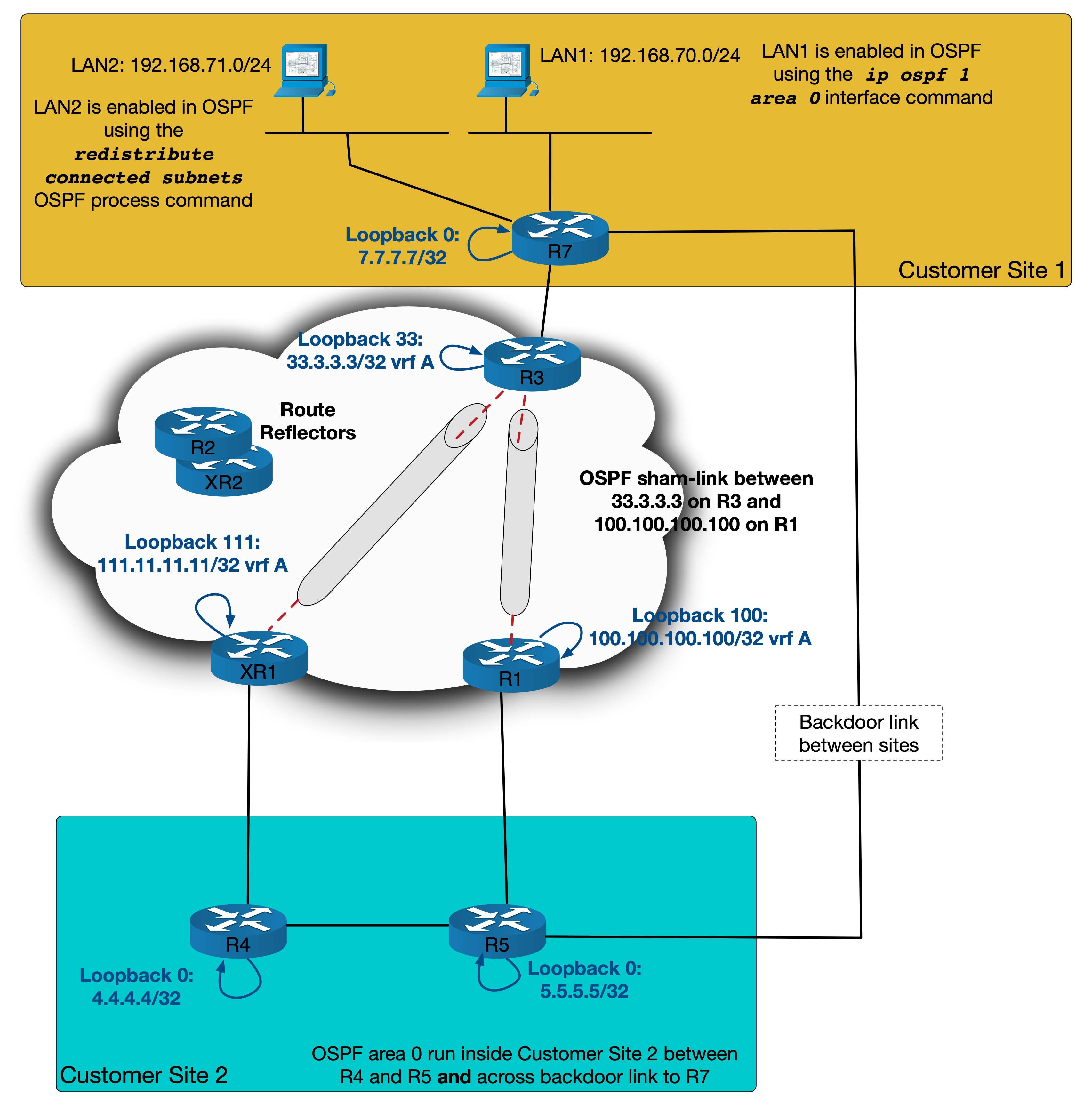
We can now test to see that if XR1 is lost, traffic will still follow the same path.
R4#conf t
Enter configuration commands, one per line.  End with CNTL/Z.
R4(config)#interface gi1.411
R4(config-subif)#shut
R4(config-subif)#do
%OSPF-5-ADJCHG: Process 1, Nbr 11.11.11.11 on GigabitEthernet1.411 from FULL to
  DOWN, Neighbor Down: Interface down or detached
R4(config-subif)#do trace 192.168.71.1 source loopback 0
Type escape sequence to abort.
Tracing the route to 192.168.71.1
VRF info: (vrf in name/id, vrf out name/id)
  1 10.4.5.5 6 msec 5 msec 4 msec
  2 10.1.5.1 5 msec 7 msec 8 msec
  3 10.1.2.2 [MPLS: Labels 16/46 Exp 0] 10 msec 17 msec 11 msec
  4 10.3.7.3 [MPLS: Label 46 Exp 0] 10 msec 6 msec 7 msec
  5 10.3.7.7 13 msec *  13 msec
R4(config-subif)#
R1 is now acting as a redundant link out of Site 2. Depending the LSA types, you could even adjust which of XR1 or R1 is the primary exit for Site 2 by adjusting the costs of the sham links! As with nearly anything that requires a full-mesh, scalability could become an issue but for our purposes here it works well.
Sham-links aren’t the most widely used tools across Service Providers but hopefully this blog has given some insight into how they work and what to consider to avoid some possible pitfalls. Are there any alternate solution you can see that might work? I’m always keen to hear alternate ideas or comments. I came across this scenario whilst working through an INE lab, so if you haven’t seen ine.com you should definitely check them out! Thank you for reading and until next time.
IVE ARP’d on for too long
The purpose of this blog is to highlight how different platforms respond to ARP requests and to explore some strange default operations on Juniper IVE VPN platforms. This quirk was found during a datacentre migration, during which the top-of-rack/first-hop device changed from a Cisco IOS 6500 environment to a Nexus Switching environment. The general setup looks like this and follows an example customer with a Shared IVS setup:

In order to understand this scenario, it’s important to know what the Juniper IVE platform is and how it provides its VPN services. To that end, I’ll give a brief overview of the platform before looking at the quirk.
IVE Platform
The Juniper 6500 IVE (Instant Virtual Extranet) platform, is a physical appliance that offers customers a unique VPN solution linking to their MPLS network. Once connected, a home worker will be connected to their corporate MPLS network just as if they were at a Branch Office.
(In order to avoid confusion between the Juniper 6500 IVE and the Cisco 6500 L3 switch -which also plays an important role in this setup but is a very different kind of device – I will just use the term IVE to refer to the Juniper platform)
IVE Ports
As you can see from the digram above, an IVE appliance has an external port and an internal port.
The external port, as its name implies, is typically assigned a public IP address. It also has virtual ports, which are analogous to sub-interfaces, each with their own IPs. Each of these virtual ports links to an individual customers VPN platform, or a shared VPN platform that holds multiple customer solutions. A common design involves placing a firewall in between the external interface and the internet. This allows the virtual interfaces to share the same subnet as the main external interface. Customer public IPs are destination NAT’d inbound (or MIP’d if you’re using a Juniper firewall) to their corresponding virtual IPs.
The internal port, similarly services multiple customers. This port can be thought of as a trunk port, whereby each VLAN links to an individual customers VRF, typically with an SVI as the gateway – sometimes used with HSRP or other FHRP.
Shared or Dedicated
Customers can have either a Shared or Dedicated VPN solution. These solutions are called IVS’s (or Instant Virtual Systems). You can have multiple IVS’s on a single IVE appliance.
Shared IVS Solutions represent a single multi-tenant IVS. Basically, multiple customers connect to the same IVS and are segmented by allocating them different sign-in pages and connection policies. Options are more limited than having a Dedicated IVS but can be more cost effective.
Dedicated IVS solutions give customers more flexibility. They can have more connected users and added customisation such as 2FA and multiple realms.
When an IVS is created it needs to link to the internal port. To do this one or more VLANs can be assigned. If the platform is Dedicated, only a single VLAN needs to be assigned – namely that of the customer. This VLAN will link to an SVI in the customers VRF. If the platform is Shared, multiple the VLANs are assigned – one per customer. However in this case, a default VLAN will need to be assigned for when the IVS needs to communicate on a network that is independent from any of its individual customers. Typically the Shared Authentication VLAN is used for this.
But what is the Shared Authentication VLAN? This leads to the next part of the setup… how users authenticate.
Authentication
When a VPN user logins in from home and authenticates, the credentials they enter on the sign-in page with need to be… well… authenticated. Much like the IVS solutions themselves, there are both Shared and Dedicated options.
Customers can have their own LDAP or RADIUS servers within their MPLS networks. In this case the IVE will make a request to this LDAP when a user connects. This is called Dedicated Authentication.
Alternatively, the Service Provider can offer a Shared Authentication solution. This alleviates the customer from having to build and maintain their own LDAP servers by utilising a multi-tenant platform managed by the Provider. The customer supplies the user details, and the Service Provider handles the rest.
Shared Authentication is typically used for Shared IVS’s. In order to connect to the Shared Authentication Server, a Shared IVS will allocate a VLAN – alongside all of its customer VLANs – on the internal trunk port. This links to the Providers network (for example an internal VRF or VLAN) where the Shared Authentication servers reside. It is this VLAN that is assigned as the default VLAN for the Shared IVS.
The below screenshot is taken from the Web UI of the IVE platform. It shows some of the configuration for a Shared IVS (namely IVS123). It uses a default VLAN called Shared_Auth_Network as noted by the asterisk in the bottom right table:
We’re nearly ready to look at the quirk. There is just one last thing to note regarding how a Shared IVS Platform, like IVS123, communicates with one of its customers Authentication Servers.
Here is the key sentence to remember: When a Shared IVS platform communicates with any authentication server (shared or dedicated), it will use its Shared Auth VLAN IP as the source address in the IP packet.
This behaviour seems very counterintuitive and I’m not sure why the IVS wouldn’t use the source IP of the VLAN for that customer IVS.
Whatever the reason for this behaviour, the result is that packets sourced from a Shared IVS Platform communicating to one of its customer’s Dedicated authentication servers, will be sending packets with a source IP of the Shared Auth VLAN. But such a customer isn’t using Shared Auth. Their network doesn’t know or care about the Shared Auth environment. So when their Dedicated LDAP server receives an authentication request from the IVE, it sees the source IP address as being from this Shared Auth VLAN.
The solution, however, is easy enough (barring any IP overlaps)… The customer simply places a redistributed static route into its VRF pointing any traffic to this Shared Auth subnet back to their internal port of the IVE.
To understand this better, let’s take a look at a diagram of the setup as a user attempts to connect:

Now we are equipped to investigate the quirk, which looks at a customer on a Shared IVS platform, but with Dedicated LDAP Authentication Servers.
The quirk
As mentioned earlier, this quirk follows a migration of an IVE platform from an environment using Cisco IOS 6500s switches to an environment using Cisco Nexus switches.
In the both environments, trunk ports connect to the internal IVE ports with SVIs acting as gateways. The difference comes in the control and dataplane that were used. The original IOS environment was a standard MPLS L3VPN network. The Nexus environment was part of a hierarchical VxLAN DC Fabric. Leaf switches connected direct to the IVEs and implemented anycast gateway on the SVIs. Prefix and MAC information was communicated over the EVPN BGP address family and ASR9k DCIs acted as border-leaves terminating the VTEPs, which were then stitched into the MPLS core.
The key difference however, isn’t in the overlays or dataplane protocols being used. The key is how each ToR device responds to ARP…
Once the move was completed and the IVE was connected to the Nexus switches everything seemed fine at first glance. Users with Dedicated IVS’s worked. Users on Shared IVS’s who utilised the Shared Auth server could also login and authenticate correctly. However a problem was found when checking any customer who had a VPN solution configured on a Shared IVS platform with Dedicated Authentication. Despite the customer login page showing up (implying that the public facing external side was working), authentication requests to their Dedicated Auth Servers were failing.
Below shows the Web UI output of a test to connect to our example customers LDAP servers at 192.168.10.10.
As we searched for a solution to this problem, we had to keep in mind how a Shared IVS Platform makes Auth Server requests…
The search
Focusing on just one of the customers on the Shared platform, we first checked how far a trace would get from the IVE to the Dedicated Auth Server. We found pretty quickly that the trace would not even reach the first hop – that is, the anycast gateway IP that was on the SVI of the Nexus leaf switch.
However when checking from the Nexus, both routing and tracing, we saw we could reach the Dedicated Auth Server fine – as long as we sourced from the right VRF.
nexus1# sh ip route vrf CUST_A | b 192.168.10.10 | head lines 5
192.168.10.0/24, ubest/mbest: 2/0
*via 172.16.24.34 %default, [20/0], 7w2d, bgp-65000, external, tag 500
    (evpn) segid: 12345 tunnelid: 0xc39dfe04 encap: VXLAN

*via 172.16.24.33 %default, [20/0], 7w2d, bgp-65000, external, tag 500
    (evpn) segid: 12345 tunnelid: 0xc39dfe05 encap: VXLAN

nexus1# traceroute 192.168.10.10 vrf CUST_A
traceroute to 192.168.10.10 (192.168.10.10), 30 hops max, 40 byte packets
1 172.16.24.33 (172.16.24.33) 1.455 ms 1.129 ms 1.022 ms
2 172.16.20.54 (172.16.20.54) 6.967 ms 6.928 ms 6.64 ms
3 10.11.2.3 (10.11.2.3) 8.002 ms 7.437 ms 7.92 ms
4 10.24.4.1 (10.24.4.1) 6.789 ms 6.683 ms 6.764 ms
5 * * *
6 192.168.10.10 (192.168.10.10) 12.374 ms 0.704 ms 0.62 ms
This led us to check the Layer 2 between the switch and the IVE. We did this by checking the ARP table entries on the IVE. We immediately found that there were no ARP entries to be found for the ToR SVI for any customer on a Shared Platform with a Dedicated Authentication setup.
The output below shows the ARP table as seen from the console of the IVE. Note the incomplete ARP entry for 172.16.20.33, the SVI on the Nexus for our example customer.
(As a quick aside, you may notice that the HWAddress of the Nexus is showing as 11:11:22:22:33:33. This is due to the fabric forwarding anycast-gateway-mac 1111.2222.3333 command being configured.)
Please choose from among the following options:
1. View/Set IP/Netmask/Gateway/DNS/WINS Settings
2. Print Routing Table
3. Print ARP Cache
4. Clear ARP Cache
5. Ping to a Server
6. Trace route to a Server
7. Remove Routes
8. Add ARP entry
9. View cluster status
10. Configure Management port (Enabled)

Choice: 3
Address       HWtype  HWaddress          Flags Mask  Iface
172.16.31.1   ether   11:11:22:22:33:33   C          int0.2387
10.101.23.4   ether   11:11:22:22:33:33   C          int0.1298
192.168.77.1  ether   11:11:22:22:33:33   C          int0.2347
172.16.20.33          (incomplete)                   int0.
So there is no ARP entry. But logically this appears to be more or less the same layer 2 segment when it connected to the 6500. So what gives?
It turns out that 6500s and Nexus switches respond to ARP requests in different ways. The process on the 6500 is fairly standard and works as follows:
But a Nexus will not respond to an ARP request if the source IP is from a subnet that it doesn’t recognise:
In our example case, the Nexus switch does not recognise 10.10.10.10 as a valid source IP for the receiving interfaces (which has IP 172.16.20.33). It sees it as off-net. We could also see the ARP check failing by using debug ip arp packet on the switch.
So what’s the solution? There are a couple of ways to tackle this. We could add a static ARP entry on the IVE, but this could be cumbersome if new needed to add it for each Shared IVS. Alternatively, we could add a secondary IP to the subnet on the SVI…
The Work
Adding a secondary IP is fairly straight forward. The config would be as follows:
nexus1# sh run interface vlan 2301
!
interface Vlan2301
description Customer_A
no shutdown
bandwidth 2000
vrf member CUST_A
no ip redirects
ip address 172.16.20.33/29
ip address 10.10.10.11/31 secondary
fabric forwarding mode anycast-gateway
A /31 works well in this case, encompassing only the IPs that are needed (namely 10.10.10.10 and 10.10.10.11) . This allows the ARP request to pass the aforementioned check that the Nexus performs. From here the MAC entries began to show up and connectivity to the Shared Auth Server began to work.
Please choose from among the following options:
1. View/Set IP/Netmask/Gateway/DNS/WINS Settings
2. Print Routing Table
3. Print ARP Cache
4. Clear ARP Cache
5. Ping to a Server
6. Trace route to a Server
7. Remove Routes
8. Add ARP entry
9. View cluster status
10. Configure Management port (Enabled)

Choice: 3
Address       HWtype  HWaddress          Flags Mask   Iface
172.16.31.1   ether   11:11:22:22:33:33   C           int0.2387
10.101.23.4   ether   11:11:22:22:33:33   C           int0.1298
192.168.77.1  ether   11:11:22:22:33:33   C           int0.2347
172.16.20.33  ether   11:11:22:22:33:33   C           int0.2301
So this raises the question of whether or not this behaviour is desired. Should a device responding to an ARP request, check the source IP? I’d tend to lean in favour of this type of behaviour. It adds extra security and besides, it’s actually the behaviour of the IVE that is strange in this case. One would think that the IVS would use the source IP of the connecting customers subnet, instead of that of the Shared Auth VLAN. The behaviour certainly is unorthodox but finding a solution to this problem highlights some of the interesting scenarios that can arise when working with different vendors and operating systems.
I hope you’ve enjoyed the read. I’m always open to alternate ideas or general discussion so if you have any thoughts, let me know.
Peering into the Future
Network automation is becoming more and more ubiquitous these days. Configuration generation is a good example of this – why spend time copy and pasting from prepared templates if a script can do it for you?
This small blog introduces the first python script to be released on netquirks. The script is called PeerPal and it automates the creation of Cisco eBGP peering configuration by referencing input from both a config file and details gather by utilising the peeringdb.com API. This serves as a good example of how network automation can make performing regular tasks faster, with fewer errors and more consistency.
The GitHub repo be found here.
It works by taking in a potential peers autonomous system number and checking with Peering DB to find which Internet Exchanges both your ASN and theirs have common presence. A list is then presented, one for IPv4 then one for IPv6, allowing you to select which locations to generate the peering config for. It can do this for either IOS or XR format. It reads the neighbors IP, prefix limits and even IRR descriptions from Peering DB and integrates them into the final output.
Other specifics of the peering, like your ASN, neighbor groups, MD5 passwords, ttl-security or what the operating system format should be, are all stored in a local config file. This can be customised per Internet Exchange.
The best way to demonstrate the script is to give a quick example. Let’s say the ISP netquirks (ASN 1234) wants to peer with ACME (ASN 5678). The script is run like this:
myhost:peerpal Steve$ python3 ./peerpal.py -p 5678
The following are the locations where Netquirks and ACME have
common IPv4 presence:
(IPs for ACME are displayed)
1: LINX LON1 - 192.168.101.1
2: CATNIX - 10.10.1.50
3: DE-CIX Frankfurt - 172.16.1.90,172.16.1.95
4: IXManchester - 10.11.11.25
5: France-IX Paris - 172.16.31.1,172.16.31.2
6: DE-CIX_Madrid - 192.168.7.7
Please enter comma-seperated list of desired peerings (e.g. 1,3,5)
or enter 'n' not to peer over IPv4:
The script first lists the Exchange names and their IPv4 IPs. Enter the Exchanges you want to peer at, and then do the same for IPv6…
myhost:peerpal Steve$ python3 ./peerpal.py -p 5678
The following are the locations where Netquirks and ACME have
common IPv4 presence:
(IPs for ACME are displayed)
1: LINX LON1 - 192.168.101.1
2: CATNIX - 10.10.1.50
3: DE-CIX Frankfurt - 172.16.1.90,172.16.1.95
4: IXManchester - 10.11.11.25
5: France-IX Paris - 172.16.31.1,172.16.31.2
6: DE-CIX_Madrid - 192.168.7.7
Please enter comma-separated list of desired peerings (e.g. 1,3,5)
or enter 'n' not to peer over IPv4: 2,4

The following are the locations where Netquirks and ACME have
common IPv6 presence:
(IPs for ACME are displayed)
1: LINX LON1 - 2001:1111:1::50
2: CATNIX - 2001:2345:6789::ca7
3: DE-CIX Frankfurt - 2001:abc:123::1,2001:abc:123::2
4: IXManchester - 2001:7ff:2:2::ea:1
5: France-IX Paris - 2001:abab:1aaa::60,2001:abab:1aaa::61
6: DE-CIX_Madrid - 2001:7f9:e12::fa:0:1
Please enter comma-separated list of desired peerings (e.g. 1,3,5)
or enter 'n' not to peer over IPv6: 6
The output produced looks like this:
IPv4 Peerings:
****************
The CATNIX IPv4 peerings are as follows:
=============================================================
Enter the following config onto these routers:
cat-rtr1.netquirks.co.uk

IOS CONFIG
----------
router bgp 5678
 neighbor 10.10.1.50 remote-as 1234
 neighbor 10.10.1.50 description AS-ACME
 neighbor 10.10.1.50 inherit peer-session EXTERNAL
 address-family ipv4 unicast
  neighbor 10.10.1.50 activate
  neighbor 10.10.1.50 maximum-prefix 800 90 restart 60
  neighbor 10.10.1.50 inherit peer-policy CATNIX

The IXManchester IPv4 peerings are as follows:
=============================================================
Enter the following config onto these routers:
mchr-rtr1.netquirks.co.uk
mchr-rtr3.netquirks.co.uk

XR CONFIG
----------
router bgp 5678
 neighbor 10.11.11.25
  remote-as 1234
  use neighbor-group default_v4_neigh_group
  ttl-security
  description AS-ACME
  address-family ipv4 unicast
   maximum-prefix 800 90 restart 60

IOS CONFIG
----------
router bgp 5678
 neighbor 10.11.11.25 remote-as 1234
 neighbor 10.11.11.25 description AS-ACME
 neighbor 10.11.11.25 inherit peer-session peer-sess-mchr4
 neighbor 10.11.11.25 ttl-security hops 1
 address-family ipv4 unicast
  neighbor 10.11.11.25 activate
  neighbor 10.11.11.25 maximum-prefix 800 90 restart 60
  neighbor 10.11.11.25 inherit peer-policy peer-pol-mchr4

IPv6 Peerings:
****************

The DE-CIX_Madrid IPv6 peerings are as follows:
=============================================================

IOS CONFIG
----------
router bgp 1042
 neighbor 2001:7f9:e12::fa:0:1 remote-as 1234
 neighbor 2001:7f9:e12::fa:0:1 description AS-ACME
 neighbor 2001:7f9:e12::fa:0:1 peer-group Mad1-6
 neighbor 2001:7f9:e12::fa:0:1 ttl-security hops 1
 address-family ipv6 unicast
  neighbor 2001:7f9:e12::fa:0:1 activate
  neighbor 2001:7f9:e12::fa:0:1 maximum-prefix 40 90 restart 60
From the output you can see that there are different specifics based on the internet exchange. Madrid uses ttl-security and peer-groups, whereas CATNIX doesn’t have ttl-security and uses peer session and policy templates. All of these specifics are stored in a local config file:
[DEFAULT]
as = 1234
op_sys = xr
ttl_sec = true
xr_neigh_grp_v4 = default_v4_neigh_group
xr_neigh_grp_v6 = default_v6_neigh_group
ios_neigh_grp_v4 = default_v4_peer_group
ios_neigh_grp_v6 = default_v6_peer_group

[CATNIX]
routers = cat-rtr1.netquirks.co.uk
op_sys = ios
ios_neigh_grp_v4 = EXTERNAL,CATNIX
ios_neigh_grp_v6 = EXTERNAL,CATNIX6
ttl_sec = false

[IXManchester]
routers = mchr-rtr1.netquirks.co.uk,mchr-rtr3.netquirks.co.uk
op_sys = both
ios_neigh_grp_v4 = peer-sess-mchr4,peer-pol-mchr4
ios_neigh_grp_v6 = peer-sess-mchr6,peer-pol-mchr6

[France-IX Paris]
xr_neigh_grp_v4 = FRANCE-NEIGH-IX
xr_neigh_grp_v6 = FRANCE-NEIGH-IXv6
ttl_sec = false

[Exchange_Number_1250]
as = 1042
op_sys = ios
ios_neigh_grp_v4 = Mad1-4
ios_neigh_grp_v6 = Mad1-6
correction = DE-CIX_Madrid
The script generally follows the structure of reading from the more specific sections first. If an IX section contains a characteristic like ttl-security, the config for that exchange will use that characteristic. If it is absent, the config will fall back on the DEFAULT section. There are a couple of exceptions to this and full details can be found in the README file on the repo. The script can also specify the routers to put the config onto and show the name of an Internet Exchange if Peering DB doesn’t have one set (DE-CIX_Madrid is an example of this as shown above). Again, full details are in the README.
This gives a brief introduction to PeerPal. It’s not a revolutionary script by any means but will hopefully come in handy for anyone working on peering or BGP configurations on a regular basis. Future planned features include pushing the actual config to the routers and conducting automated checks to make sure that prefixes and traffic levels adhere to your peering policy – watch this space.
So feel free to clone the repo and give it a go. Thoughts and comments welcome as always.
The A to Zabbix of Trapping & Polling
Monitoring is one of the most crucial parts to running any network. There are many tools available to perform network monitoring, some of which are more flexible than others. This quirk looks at the Zabbix monitoring platform – more specifically, how you use combined SNMP polling and trapping triggers to monitor an IP network, based on Zabbix version 3.2.
The blog assumes you’re already familiar with the workings of Zabbix. However if you aren’t, the follow section gives a whistle-stop tour, from the perspective of discovering and monitoring network devices using SNMP. If you are already familiar with Zabbix, skip to The quirk section below.
Zabbix – SNMP Monitoring Overview
Zabbix can do much (much) more than I’ll outline here, but if you’re not familiar with it, I’ll describe roughly how it works in relation to this quirk.
The Zabbix application is installed on a central server with the option of having one or more proxy servers that relay information back to the central server. Zabbix has the capability to monitor a wide range of environments from cloud storage platforms to LAN switching. It uses a variety tools to accomplish this but here I’ll focus on its use of SNMP.
Anything that can be exposed in an SNMP MIB can be detected and monitored by Zabbix. Examples of metrics or values that you might want to monitor in a networking environment include:
- Interfaces states
- Memory and CPU levels
- Protocol information (neighbors IPs, neighborship status etc)
- System uptime
- Spanning-Tree events
- HA failover events
In Zabbix these metrics/values are called items. A device that is being monitored is referred to as a host.
Zabbix monitors items on hosts by both SNMP polling and trapping. It can, for example, poll a switch’s interfaces every 5 minutes and alert if a poll response comes back stating the interface is down (the ifOperStatus OID is good for this). Alternatively an item can be configured to listen for traps. If a switch interface drops, and that switch sends an SNMP trap (either to the central server or one of its proxies), Zabbix can pick this up and trigger an alert.
So how is it actually configured and setup?
The configuration of Zabbix to monitor SNMP follows these basic steps. Zabbix specific terms have been coloured red:
- Add a new host into Zabbix – including its IP, SNMP community and name. The device in question will need to have the appropriate read-only SNMP community configured and have trapping/polling allowed to/from the Zabbix address.

- Configure items for that host – An item can reference a poll (e.g. poll this device for its CPU usage) or a trap (e.g. listen for an ‘interface up/down’ trap).
- Configure triggers that match particular expressions relating one or more items. For example a trigger could be configured to match against the ‘CPU usage’ item receiving a value (though polling) of 90 or more (e.g. 90% CPU). The trigger will then move from an OK state to a PROBLEM state. When the trigger clears (more on that below) it will move from a PROBLEM state back to an OK state.

- Configure actions that correspond triggers moving to a PROBLEM state – options depend on the severity level of the trigger but could be something like sending an email or integrating with the API of something like PagerDuty to send an SMS
This process is pretty simple on the face of things, but what happens if you have 30 switches with 48 interfaces each? You couldn’t very well configure 30×48 items that monitor interfaces states. That’s a lot of copy and pasting!
Thankfully, Zabbix has two features that allow for large scale deployments like this:
Templates – Templates allow you to configure what are called prototype items and triggers. These prototypes are bundled all into one common template. You can then apply that template to multiple devices and they will all inherit the items and triggers without them needing to be configured individually.
Low Level Discovery – LLD allows you to discover multiple items based on SNMP tables. For example if you create an LLD rule with the SNMP OID ifIndex (1.3.6.1.2.1.2.2.1.1) as the Key, Zabbix will walk that table and discover all of its interfaces. You can then take the index of each row in the table and use it to create items and triggers based on other SNMP tables. For example after discovering all the rows of the ifIndex table you could use the SNMP Index in each row to find the ifOperStatus of each of those interfaces. It doesn’t matter if the host has 48 or 8 interfaces, they will all be added using this LLD. Here’s an example of the principle using snmpwalk:

Now this is a very high level overview of Zabbix. I’m just giving a brief snapshot for those who haven’t worked with Zabbix.
Before mention the specifics of this quirk, I’ll go into a little more detail on how triggers work, since it plays a crucial role …
A trigger is an expression that is applied to an item and, as you might expect, is used to detect when a problem occurs. A trigger has two states: OK or PROBLEM. To detect when a problem occurs, a trigger uses an aptly named problem expression. The problem expression is basically a statement that describes the conditions under which the trigger should go off (e.g. move from OK to PROBLEM).
Examples of a problem expression could be “the last poll of interface x on switch y indicates it is down” or “the last trap received from switch y indicates interface x is down”.
Triggers also have a recovery expression. This is sort of the opposite of a problem expression. Once a trigger goes off, it will remain in the PROBLEM state until such time as the problem expression is no longer true. If the problem expression suddenly evaluates to false, the trigger will move to looking at the recovery expression (if one exists). At this point, the trigger will stay in a PROBLEM state until the recovery expression becomes true. The distinction to pay attention to here is that the even though the original condition that caused the trigger to go off is no longer true, the trigger remains in a PROBLEM state until the recovery expression is true. Most importantly, the recovery expression is not evaluated until the problem expression is false. Remember this for later.
So with all of that said. Let’s take a look at the quirk.
The quirk
This quirk explores how to configure triggers within Zabbix to use both polling and trapping to monitor a network device such as a router or switch.
To illustrate the idea I will keep it simple – interface states. Imagine a template applied to a switch that uses LLD to discover all of the interfaces using the ifIndex table.
Two items prototypes are created:
One that polls the interface state (ifOperStatus) every 5 minutes
and
One that listens for traps about interface states – either going down (for example listening for 1.3.6.1.6.3.1.1.5.3 linkDown traps) or coming up (for example listening for 1.3.6.1.6.3.1.1.5.4 linkUp traps)
The question is, how should the trigger be configured? We do not want to miss an interface that flaps. If an interface drops, we want the trigger to move to a PROBLEM state. But if our trigger is just monitoring the polling item and the interface goes down and comes back up within a polling cycle then Zabbix won’t see the flap.
To illustrate these concepts, I’ll use a diagram that shows a timeline together with what polling and trapping information is received by Zabbix. It uses the following legend:
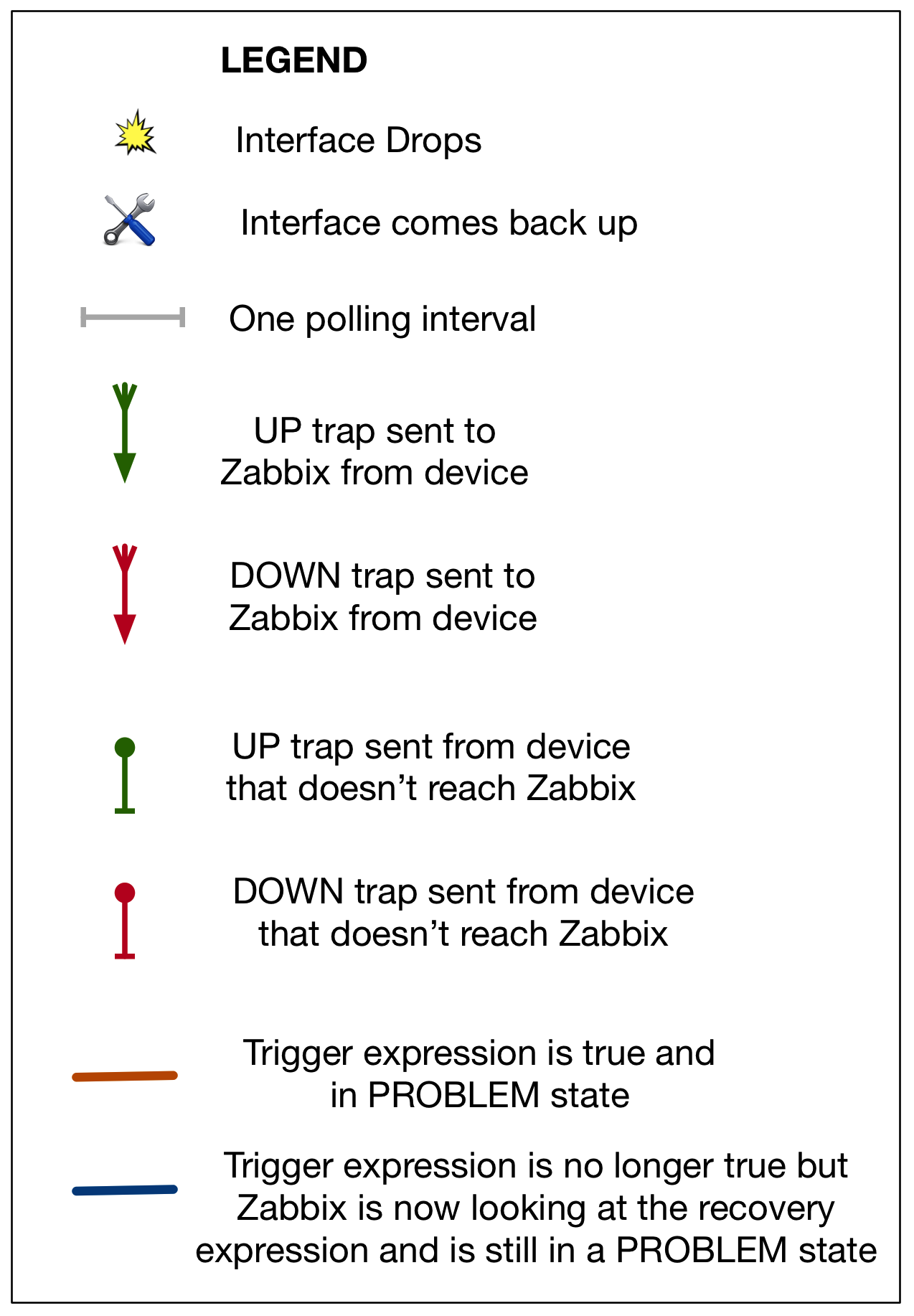
This first diagram illustrates how Zabbix could “miss” an interface flap, if it occurs between polling responses:

You can see here, that without trapping, as far as Zabbix is concerned the interface never drops.
So what if we just make our trigger monitor traps?
This also runs into trouble when you consider that SNMP runs over UDP and there is no guarantee that a trap will get through (especially if the interface drop affects routing or forwarding). Worse still, if the trap stating that the interface is down (the DOWN trap) makes it to Zabbix but the recovery trap (the UP trap) doesn’t make it to Zabbix then the trigger will never recover!

It appears that both approaches on their own have setbacks. The logical next step would be to look at combining the best of both worlds – i.e. configure a trigger that will move to a PROBLEM state if it receives a DOWN trap or a poll sees the interface as down. That way, one backs the other up. The idea looks like this:

Seems simple enough. However, the quirk arises when you realise there is still a problem with this approach …. namely, if the UP trap is missed, the trigger will still not recover.
To understand why, we’ll look at the logic of the trigger expression. The trigger expression is a disjunction – an or statement. The two parts of this or statement are:
The last poll states the interface is down
OR
The last trap received indicates the interface is down
A disjunction only requires one of the parts to be true for the whole expression to be true.
Consider this scenario: A DOWN trap is received, making the second part of the expression true. The trigger moves to a PROBLEM state. So far so good. Now image a few minutes later the interface comes back up but the UP trap is never received by Zabbix. Due to the fact that this is a disjunction, even if the last poll shows the interfaces as up, the second half of the expression is still true – as far as Zabbix is concerned that last trap it received showed the interface is down. As a result the alert will never clear (meaning the trigger will never move from PROBLEM back to OK).
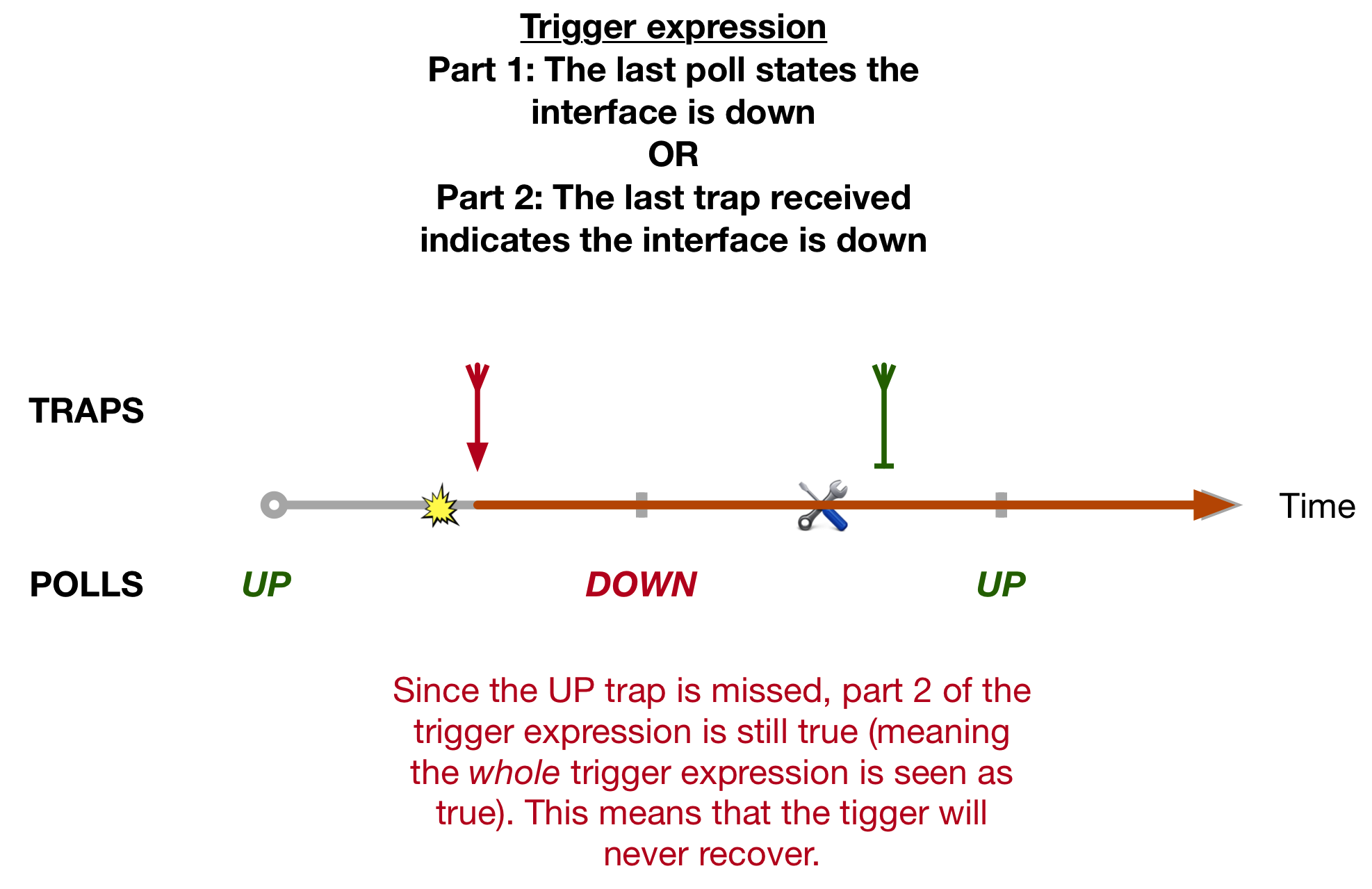
There needs to be some way to configure the combination of the two that doesn’t leave the trigger in a PROBLEM state. When searching for a solution, the Recovery Condition comes into play…
The search
To focus on finding a solution we will first look at solving the missing UP trap problem. For now, don’t worry about polling.
Let’s say we a have trigger with the following trigger expression:
The last trap received indicates the interface is down
Then clearly if the trigger has gone off and we miss the UP trap when the interface recovers, this alert will never clear. So what if we combine this, using an and statement, with something else. Something else that will, no matter what, eventually become false. Since an and statement is a conjunction, both parts will need to be true. We can then use the recovery condition to control when the trigger moves back to an OK state.
We can leverage polling for this since, if the interface is down, polling will eventually detect it. So our trigger expression changes to this:
The last trap received indicates the interface is down
AND
The last poll states the interface is up
At first this might seem counter intuitive to what we looked at above, but consider that when an interface drops and the switch sends a trap to Zabbix, stating that the interface is down, the last poll that Zabbix made to the switch should have shown the interface as up – hence both statements are true and the trigger correctly moves to a PROBLEM state.
But as soon as polling catches up and detects that the interface is down, the second part of our trigger expression with become false. This makes the whole trigger expression false (since it is a conjunction) and the trigger will recover and move back to an OK state.

Now this is obviously not good. The interface is, afterall, still down! But we can use the recovery expression to control when the trigger recovers.
Remember from earlier that if a recovery expression exists, it will be looked at once the problem expression becomes false.
We can’t just configure a recovery expression on its own, until we made the above tweak, since as long as the problem expression says true the recovery expression will still be ignored.
From here the solution is simple. Our recovery expression simply states
The last two polls that we received stated the interface was up.
This means that as soon as polling detects that the interface is down, the problem statement becomes false and the recovery expression is looked at. Now, until two polls in a row detect that the interface is up, the trigger will stay in a PROBLEM state.
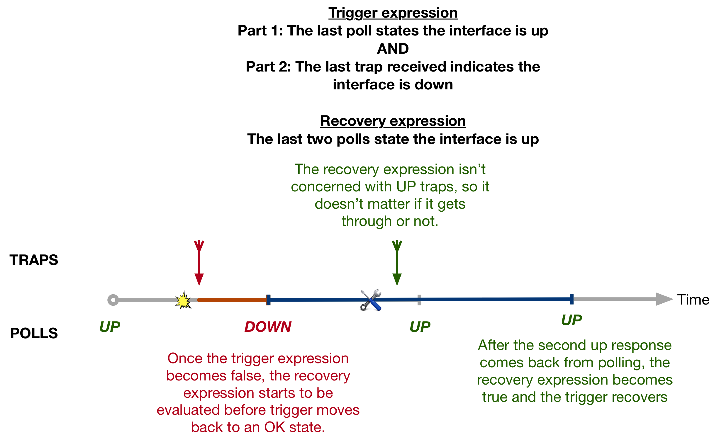
Interestingly, what we’ve essentially done is solve the missing UP trap problem, by removing the need to rely on UP traps at all! After two UP polls the trigger recovers (note the blue line of the timeline in the above diagram). You could optionally include an …or an UP trap is received to the recovery statement to make the recovery time quicker.
But there is a caveat to this case…
Consider what happens if an interface flaps within a polling cycle, meaning as far as polling is concerned, the interface never goes down. This would mean that, in the event that UP trap is missed, the problem statement will never become false. This means the trigger will never recover and we’re back to square one…

What we need is something that will inevitably cause the trigger statement to become false. Using polling doesn’t work because as we have seen, it can “miss” an interface flap.
Fortunately Zabbix has a function called nodata which can help us. The function can be found here and works as follows:
nodata(x) = 1(true) or 0(false), where x is the number of seconds where the referenced function has (true) or has not (false) received data.
To better understand this, let’s see what happens is we remove the statement The last poll states the interface is up, and replace it with one that implements this function. Our trigger statement would then become the following:
The last trap received indicates the interface is down
AND
There has been some trap data received in last x seconds (where x > bigger than the polling interval)
The second part of this conjunction is represented by trap.nodata(350) = 0 (e.g. “It is false that there has been no trap information received in the last 350 seconds” which basically means “you have received some trap information in the last 350 seconds”).
Once the 350 seconds expires that statement becomes false and the trigger moves to looking at the recovery expression. Remember our polling interval was 5 minutes, or 300 seconds.
The value x, must be at least as long as a polling interval, this will give the polling a chance to catch up as it were. Consider a scenario where x is less than a single polling interval and the interface drops just after the last poll. The nodata(x) expression will expire before the next poll comes through. When this happens, the trigger statement is false, so Zabbix will move to look at the Recovery Expression (which states that the last two polls are up). Zabbix will see the last two polls as up and trigger will recover when the interface is still down!

If x is bigger than the polling interval, polling can catch up and the trigger behaves correctly.

Now that we have solved this we can reintroduce polling into the trigger. Remember that the initial DOWN trap could still be missed. We saw that there were problems when trying to integrate polling and trapping together into a trigger’s Problem Expression, but we can easily create a single poll-based trigger.
This trigger can be relatively simple. The Problem Expression simply states that the last two polls show the interface as down. There doesn’t need to be a Recovery Expression, since when the trigger sees two UP polls it can recover without problems.
Now we’ve got another problem though. We don’t want two triggers to go off for just one event. Thankfully Zabbix has the feature of dependence. If we configure the poll-based trigger to only move to a PROBLEM state if the trap-based trigger is not in a PROBLEM state, then this poll-based trigger effectively acts as a backup to the trap-based one. I’ll explore the exact configuration of this in the work section.
Once this has been configured you’ll have a working solution that supports both polling and trapping without having to worry about alerts not triggering or clearing when they should. Let’s take a look at how this configured on the Zabbix UI.
The Work
In this section I will show screenshots of the triggers that are used in the aforementioned solution. I haven’t shown the configuration of the LLD or of any corresponding Actions (that will result in email or text messages being sent), but Zabbix has excellent documentation on the how to configure these features.
First we’ll look at the trapping configuration:

The Name field can use variables based on OIDs (like ifDesc and ifAlias) that are defined in the Low Level Discovery rule to make the trigger contain meaningful information of the affected interface. The trigger expression references the trap item that listens for interface down traps.
The trap item itself will look at the log output produced by the Zabbix snmptrapd process passing traps through an SNMPTT config file. This process parses incoming traps and creates log entries. Trap items can then match against these logs.
In this case, the item matches against log entries containing the string
“Link up on interface {#SNMPINDEX}” – which is produced when a linkup trap is received
Or
“Link down on interface {#SNMPINDEX}”}” – which is produced when a linkdown trap is received
where {#SNMPINDEX} is the index of the table entry for the ifIndex table.
In this trigger expression the trap item is referenced twice. Firstly, it matches a trap item that has the “link down” substring in it (i.e. if a down trap is received for that ifIndex). Secondly, it uses the noData = 0 (false) function – this means that “some trap data has been received in the past 350 seconds”.
This matches the pseudo-expression we have above:
The last trap received indicates the interface is down
AND
There has been some trap data received in last x seconds (where x > bigger than the polling interval).
If a trap is received stating the interface is up, the trap item will no longer contain the string “link down” – rather it will contain “link up”, so the first part will become false.
Alternative, if no trap is received in 350 second (either UP or DOWN) the second half of the AND statement will become false. The polling interval is less that 350 seconds so if the up trap is missed polling will have the chance to catch up.
Either way, the trigger will eventually look at the recovery expression. The recovery expression references the ifOperStatus item and the ifAdminStatus item.
The recovery expression basically states:
IF
The last two polls of the interface operational state is up
OR
The last poll of the administrative state of the interface is down (i.e. someone has issued ‘shutdown’ on the interface, if it’s an interface on a Cisco device)
THEN recover.
The second half of the disjunction is used to account for scenarios where an engineer deliberately shut down an interface – in which case you would not want the alert to persist.
Next we’ll look at the polling trigger:

This one is much simpler. The trigger will go off if the last two polls of the interface indicate that the operational state is down (2) AND the admin state is up (1) – meaning that it hasn’t been manually shutdown by an engineer.
Finally, the last trick to making this solution works is in the dependencies tab of this trigger prototype:

In this screen, the trap-based trigger has been selected as a dependency for the poll-based trigger. This means that the poll-based trigger will only go off if the trap-based trigger hasn’t gone of.
So that’s the work involved in configuring the actual triggers and it brings us to the end of this quirk. It demonstrates how to combine polling and trapping into Zabbix triggers to allow for consistent and correct alerting.
Zabbix has a wide range of functions and capabilities – far more than what I’ve outlined there. There may very well be another way to accomplish the same goal so as usual, any thoughts or idea are welcome.
The Friend of my Friend is my Enemy
Imagine you’re a provider routing a PI space prefix for one of your customers. Now imagine that one of your IX peers started to advertise a more specific subnet of that customer network to you. How would and how should you forward traffic destined for that prefix? This quirk looks at just a such a scenario from the point of view of an ISP that adheres to BCP38 best practice filtering policies…
The quirk
So here’s the scenario:
In this setup Xellent IT Ltd is both a customer and a provider. It provides transit for ACME Consulting but it is a customer of Provider A. ACME owns PI space and choses to implement some traffic engineering. It advertises a /23 to Xellent IT and a /24 to Provider B.
Now Provider B just happens to peer with Provider A over a public internet exchange. The quirk appears when traffic from the internet, destined to 1.1.1.1/32, enters Provider A’s network, especially when you consider that Provider A implements routing policies that adhere to BCP38.
But first, what is BCP38?
You can read it yourself here, but in short, it is a Best Current Practice document that advocates for prefix filtering to minimise threats like DDoS attacks. It does this by proposing inbound PE filtering on customer connections that block traffic whose source address does not match that of a known downstream customer network. DDoS attacks have spoofed source addresses. So if every Provider filtered traffic from their customers, to make sure that the source address was from the right subnet (and not spoofed) then these kinds of DoS attacks would disappear overnight.
To quote the BCP directly:
In other words, if an ISP is aggregating routing announcements for multiple downstream networks, strict traffic filtering should be used to prohibit traffic which claims to have originated from outside of these aggregated announcements.
BCP38 – P. Ferguson, D. Senie
To put it in diagram form, the basic idea is as follows:
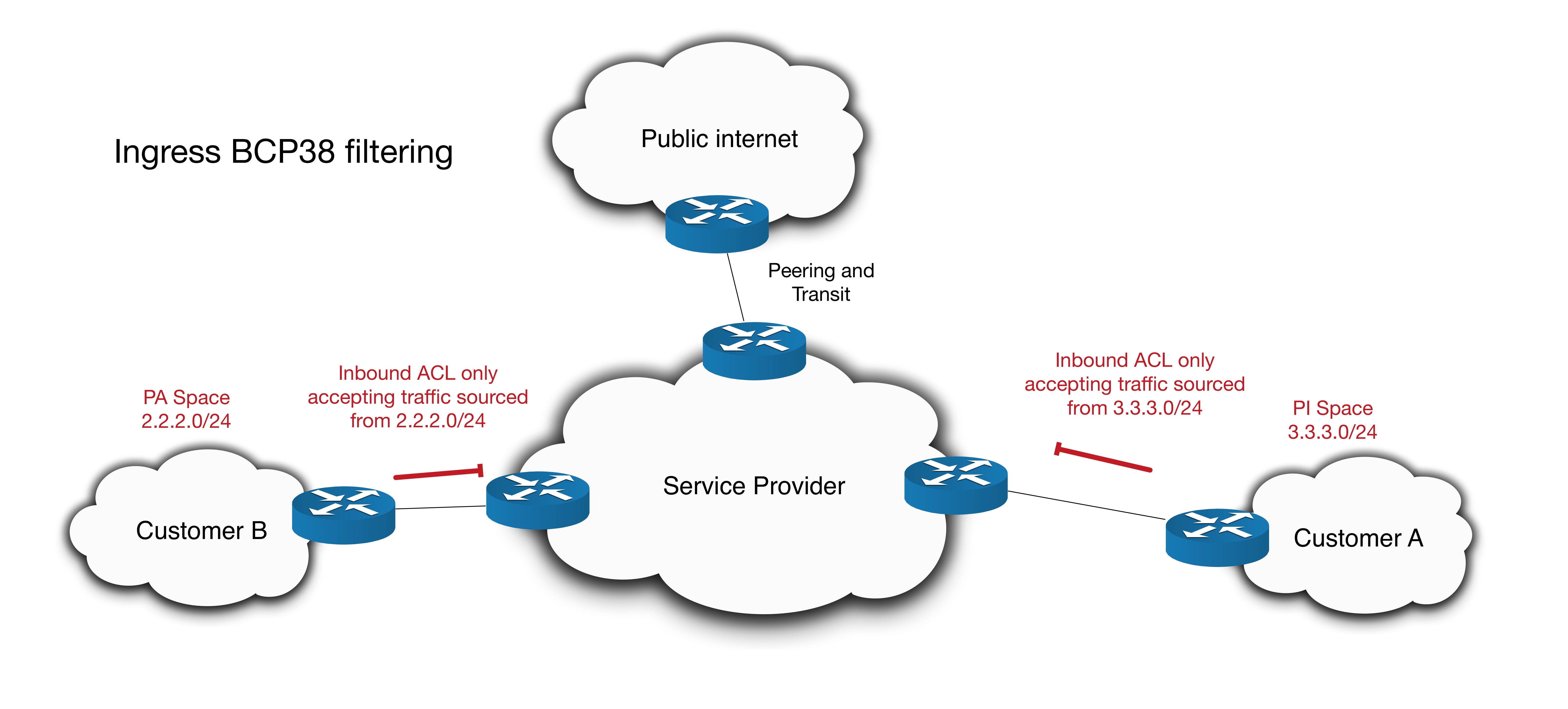
A provider can also implement outbound filtering to achieve the same result. That is to say, outbound filters can be applied at peering and transit points to ensure that the source addresses of any packets sent out come from within the customer cone of the provider (a customer cone is the set of prefixes sourced by a provider, either as PI or PA space, that makes up the address space for is customer base). This can be done in conjunction with, or instead of, the inbound filtering approach.
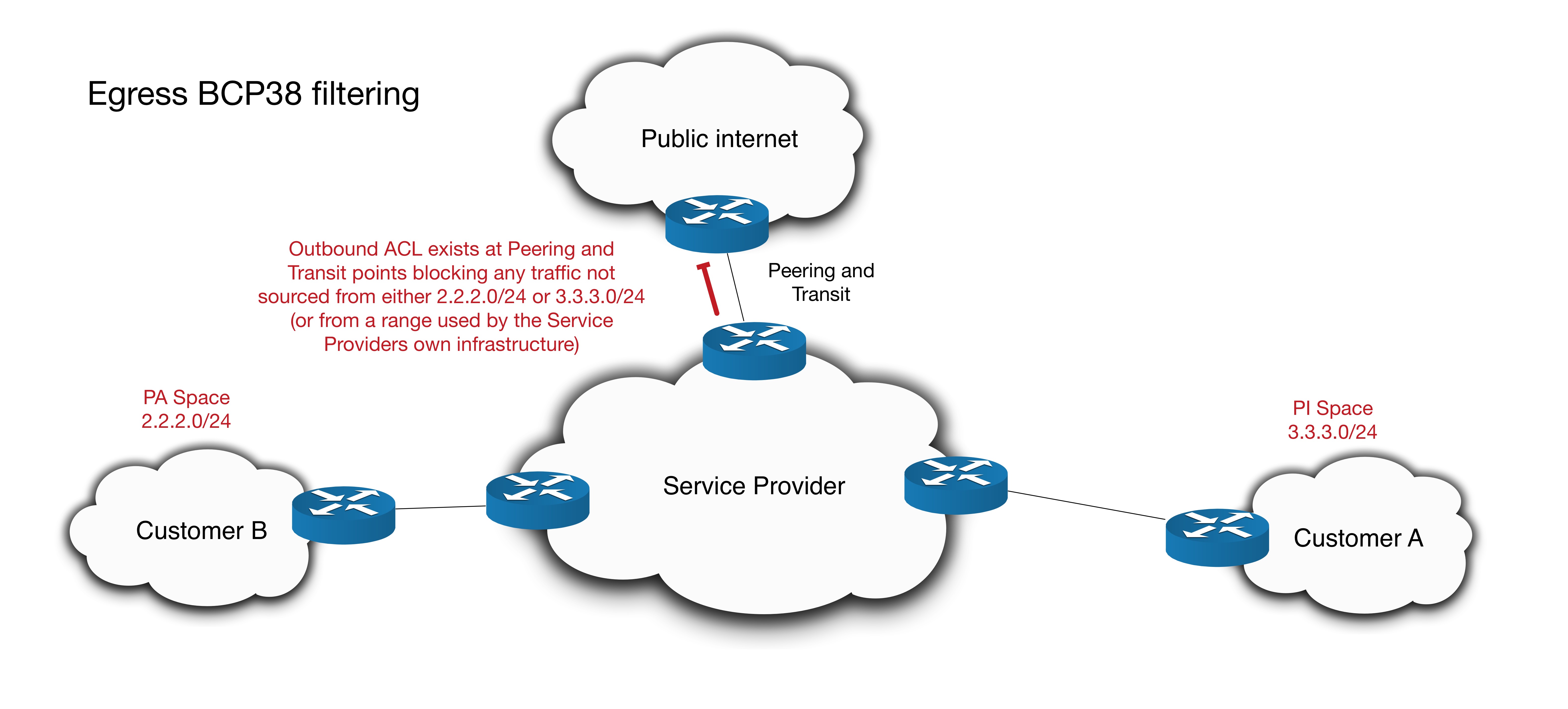
There are multiple ways a provider can build their network to adhere to BCP38. As an example, an automated tool could be built that references an RIR database like RIPE. This tool could perform recursive route object lookups on all autonomous systems listed in the providers AS-SET and build an ACL that blocks all outbound border traffic whose source address is not in that list.
Regardless of the method used, this quirk assumes that Provider A is using both inbound and outbound filtering. But as we’ll see, it is the outbound filtering that causes all the trouble… here’s the traffic flow:
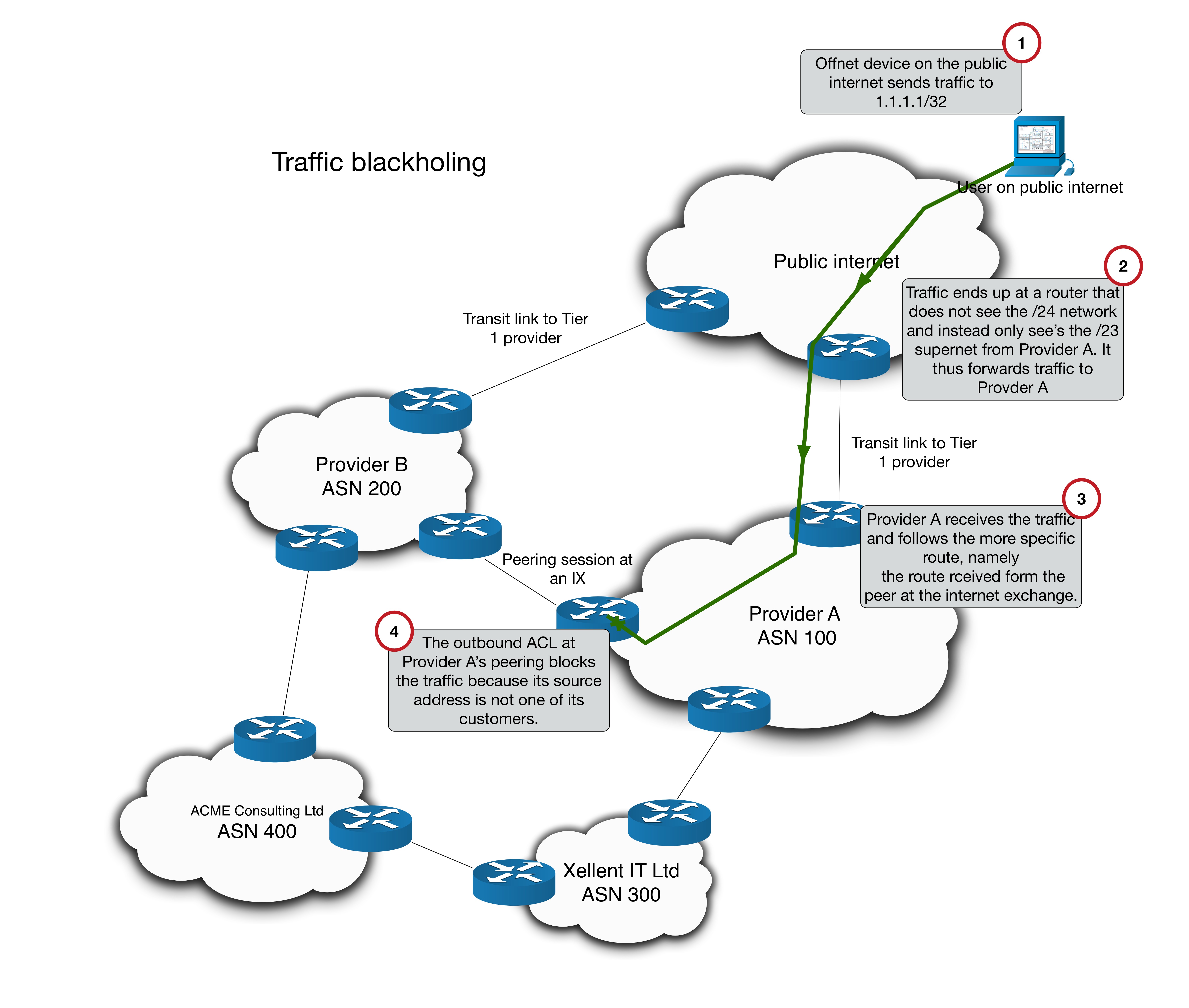
Now you might ask why the packet would follow this particular path. Isn’t Provider B advertising the more specific /24 it receives from ACME? How come the router that sent the packet to Provider A over the transit link can’t see the /24?
There are a number of reason for this and it depends on how the network of each Autonomous System along the way is designed. However, one common reason could be due to a traffic engineering service offered but Internet Providers call prefix scoping.
Prefix scoping allows a customer to essentially tell its provider how to advertise its prefix to the rest of the internet. This is done by including predetermined BGP communities in the prefix advertisements. The provider will recognise these communities and alter how they advertise that prefix to the wider internet. This could be done through something like route-map filtering on these communities.
In this scenario, perhaps Provider B is offering such a service. ACME may have chosen to attach the ‘do not advertise this prefix to your transit provider x’ community to its BGP advertisement to Provider B. As a result, the /24 prefix doesn’t reach the router connecting to Provider A over its transit link, so it forwards according to the /23.
This is just one example of how traffic can end up at Provider A. For now, let’s get back to the life of this packet as it enters Provider A.
Upon receipt of the packet destined for 1.1.1.1/32, Provider A’s border router will look in its routing table to determine the next hop. Because it is more specific, the 1.1.1.0/24 learned over peering will be seen in the RIB as the best path, not the /23 from the Xellent IT link. The packet is placed in an LSP (assuming an MPLS core) with a next hop of the border router that peers with Provider B at the Internet Exchange.
You can probably see what’s going to happen. When Provider A’s border router at the Internet Exchange tries to forward the packet to Provider B it has to pass through an outbound ACL. This ACL has been built in accordance with BCP38. The ACL simply checks the source address to make sure it is from with the customer cone of Provider A. Since the source address is an unknown public address sourced from off-net, the packet is dropped.
Now this is inherently a good thing isn’t it? Without this filtering, Provider A would be providing transit for free! However, it does pose a problem after all, since traffic for one of its customers subnets is being blackholed.
From here, ACME Consulting gets complaints from its customers that they can’t access their webserver. ACME contacts its transit providers and before you know it, an engineer at Provider B has done a traceroute and calls Provider A to ask why the final hop in the failed trace ends in Provider As network.
So where to from here? What should Provider A do? It doesn’t want to provide transit for free, and its policy states that BCP38 filtering must be in place. Let’s explore the options.
The Search
Before I look at the options available, it worth pausing here to reference an excellent paper by Pierre Francois of the Universite catholique de Louvain entitled Exploiting BGP Scoping Services to Violate Internet Transit Policies. It can be read here and describes the principles underlying what is happening in this quirk in a more high level logistical way that sheds light on why this is happening. I won’t go into exhaustive detail, I highly recommend reading the paper yourself, but to summarise, there are 3 conditions that come together to cause this problem.
- The victim Provider whose policy is violated (Provider A) receives the more specific prefix from only peers or transit providers.
- The victim Provider also has a customer path towards the less specific prefix.
- Some of the victims Providers peer or transit providers did not receive the more specific path.
This is certainly what is happening here. Provider A sees a /24 from its peer (condition 1), a /23 from its customer (condition 2) and the Transit router that forwards the packet to Provider A cannot see the /24 (condition 3). The result of these conditions is that the packet is being forwarded from AS to AS based on a combination of the more specific route and the less specific route. To quote directly from Francois’ paper:
The scoping being performed on a more specific prefix might no longer let routing information for the specific prefix be spread to all ASes of the routing system. In such cases, some ASes will route traffic falling to the range of the more specific prefix, p, according to the routing information obtained for the larger range covering it, P.
Exploiting BGP Scoping Services to Violate
Internet Transit Policies – Pierre Francois
So what options does Provider A have? How can it ensure that traffic isn’t dropped, but at the same time, make sure it can’t be abused into providing free transit for off-net traffic? Well there’s no easy answer but there are several solutions that I’ll consider:
- Blocking the more specific route from the peer
- Asking Xellent IT Ltd to advertise the more specific
- Allowing the transit traffic, but with some conditions
I’ll try to argue that allowing the transit traffic but only as an exception, is the best course of action. But before that, let’s look at the first two options.
Let’s say Provider A applies an inbound route-map on its peering with Provider B (and all other peers and transits for that matter) to block any advertised prefixes that come from its own customer cone (basically, stopping its own prefixes being advertise towards itself from a non-customer). So Provider A would see Provider B advertising 1.1.1.0/24 and recognise that it as part of Xellent ITs supernet and block it.
This would certainly solve the problem of attempting to forward the traffic out of the Internet Exchange. Unfortunately, there are two crushing flaws with this approach.
Firstly, it undermines the intended traffic engineering employed by ACME and comes will all the inherent problems that asymmetric routing holds. For example, traffic ingressing back into ACME via Xellent IT could get dropped by a session-based firewall that it didn’t go through on its way out. Asymmetric routing is a perfect example of the problems than can result from some ASes forwarding on the more specific route and others forwarding on the less specific route.
Second, consider what happens if the link to Xellent IT goes down, or if Xellent IT stops advertising the /23. Suddenly Provider A has no access to the /24 network. Provider A is, in essence, relying on a customer to access part of the internet (this is of course assuming Provider A is not relying on any default routing). This would not only undermine the dual homing of Customer B, but would also stop Provider A’s other customers reaching ACMEs services.
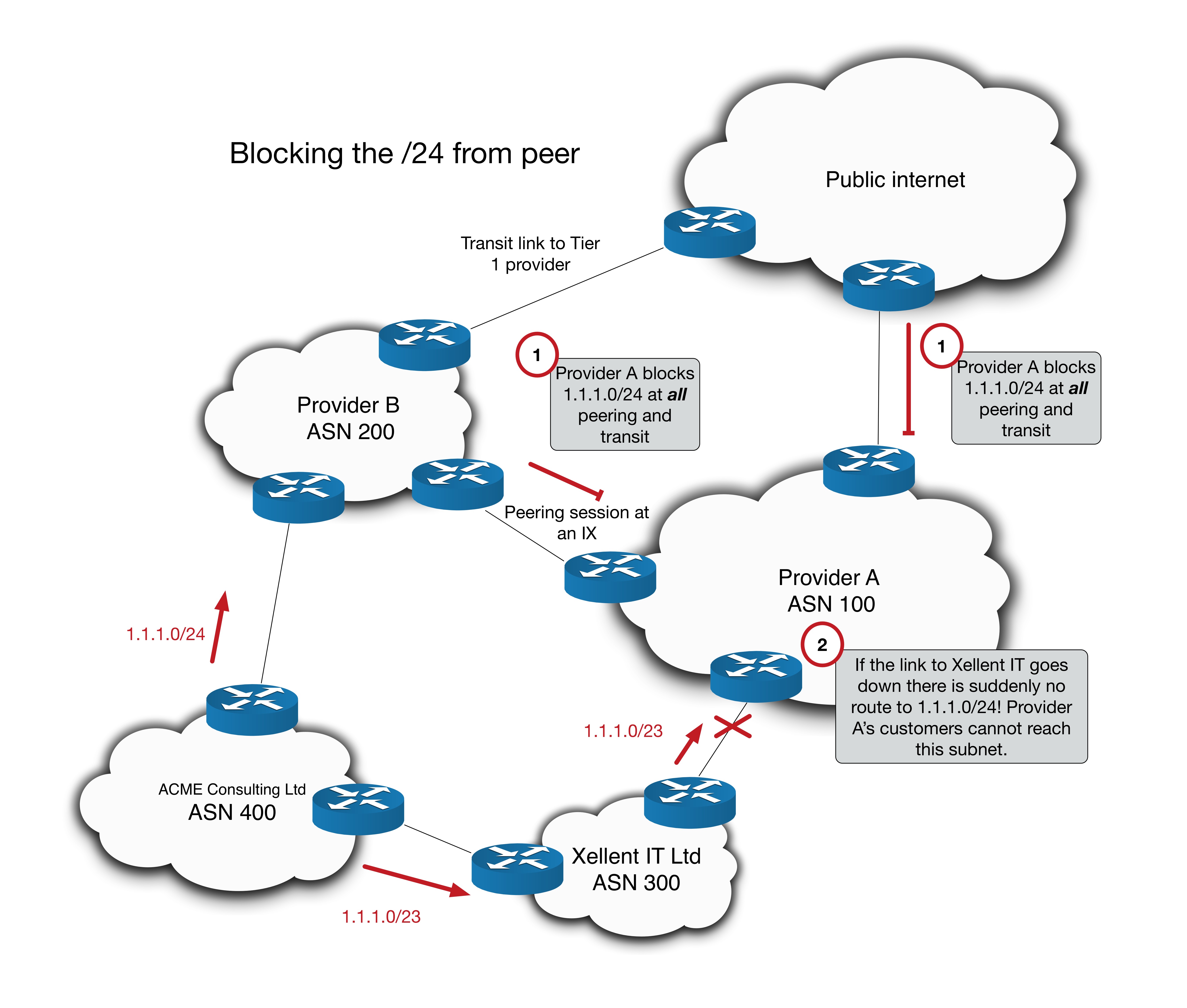
Clearly forwarding the traffic based on the less specific by blocking the more specific from the peer doesn’t solve anything. It might get through Provider A, but traffic is still being forwarding on a combination of prefix lengths and Provider A could end up denying traffic from its other customers reaching a part of the internet. Not a good look for an internet provider.
What about asking Xellent IT to advertise the more specific? Provider A could then simply prefer the /24 from Xellent IT using local preference. This approach has problems too. ACME isn’t actually advertising the /24 to Xellent IT. Xellent IT would need to ask ACME to do so, however they may not wish to impose such a restriction on their customer. The question then becomes, does Provider A have the right to make such a request? They certainly can’t enforce it.
There is perhaps a legal argument to be made that by not advertising the more specific Provider A is losing revenue. This will be illustrated when we look at the third option of allowing off-net traffic. I won’t broach the topic of whether or not Provider could approach Xellent IT and ask for advertisement of the more specific due to revenue loss, but it is certainly food for thought. For now though, asking Xellent IT to advertise the more specific is perhaps not the preferred approach.
Let’s turn to the third option, which sees Provider A adjust its border policies by adding to its BCP38 ACL. Not only should this ACL permit traffic with source addresses from its customer cone, it should also permit traffic that is destined to prefixes in its customer cone. The idea looks like this:

Now this might look ok. Off-net transit traffic to random public address (outside of Provider As customer cone) is still blocked, and ACMEs traffic isn’t. But this special case of off-net transit opens the door for abuse in a way that could cause Provider A to lose money.
Here’s how it works. For the sake of this explanation, I’ve removed Xellent IT and made ACME a direct customer of Provider A. I’ve also introduced a third service provider.
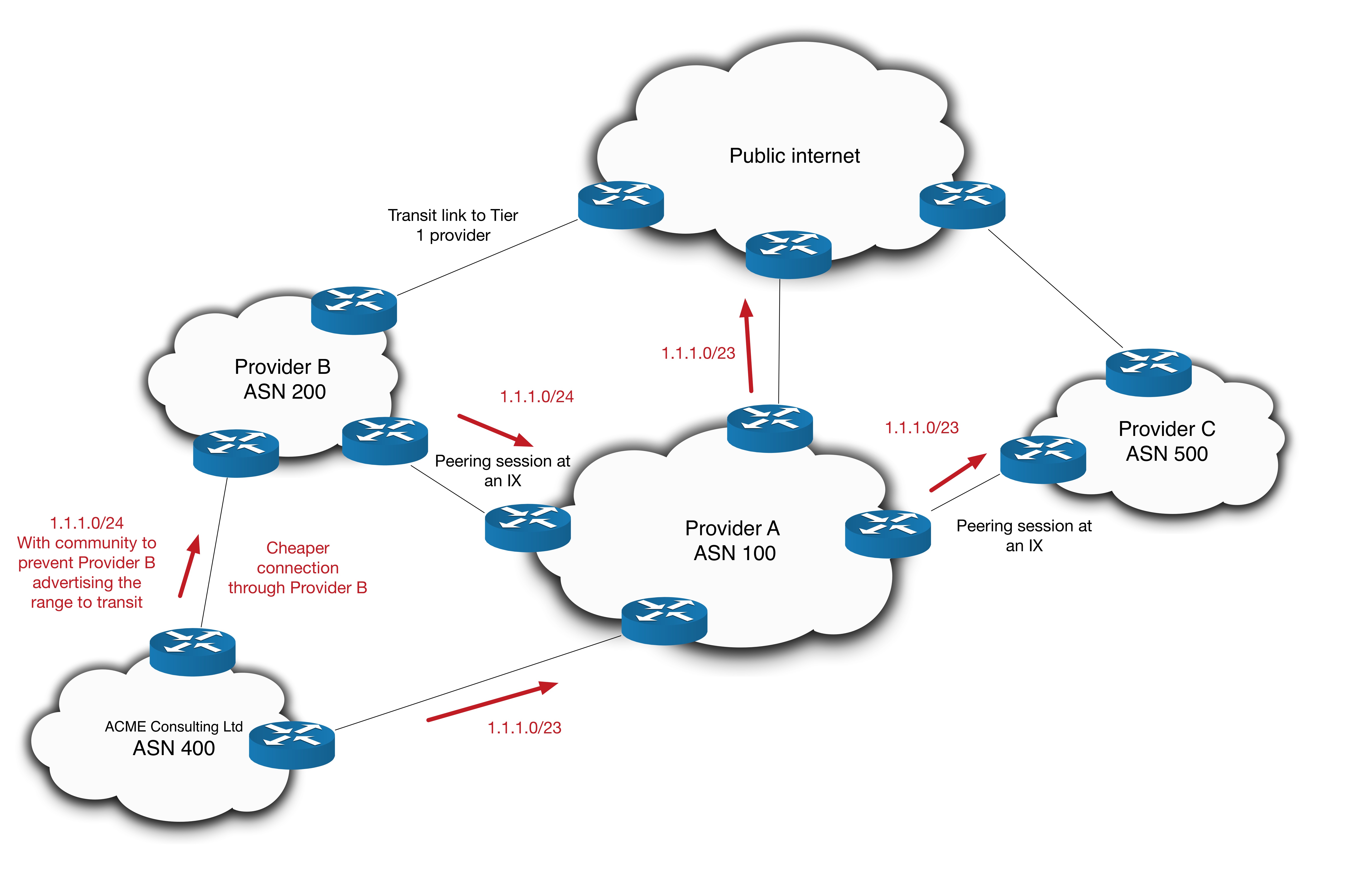
- ACME dual homes itself by buying transit from Provider’s A and B. Provider A happens to charge more.
- ACME advertises its /23 PI space to Provider A
- It’s /24 is then advertised to Provider B, with a prefix scoping attribute that tells provider B not to advertise the /24 on to any transit providers.
- As a result of this, Provider C cannot see the more specific /24. Traffic from Provider C traverses Provider A, then Provider B before arriving at ACME.
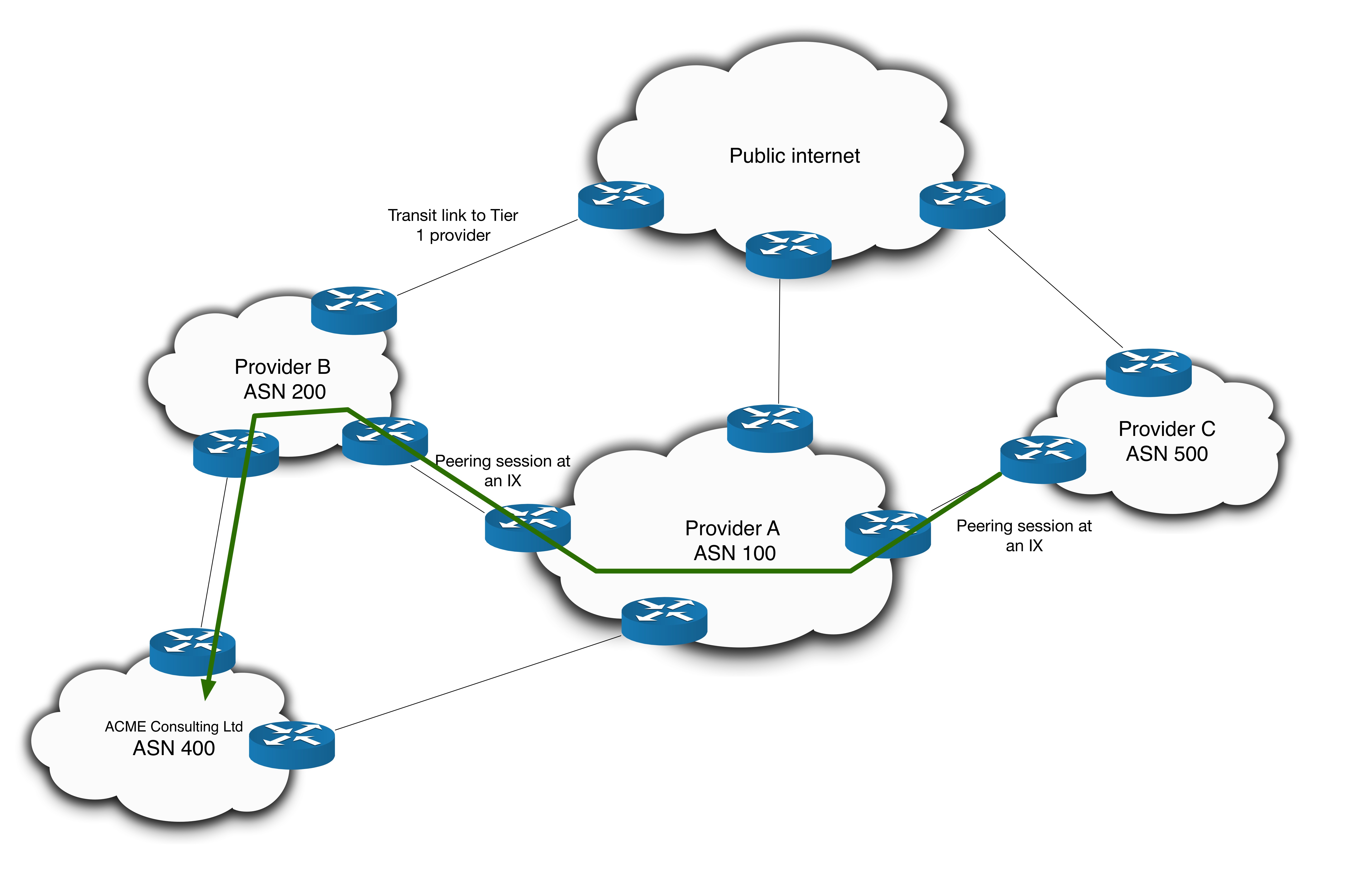
As we’ve already discussed, this violates BCP38 principles and turns Provider A into free transit for off-net traffic. But of perhaps greater importance is the loss of revenue that Provider A experiences. No one is paying for the increased traffic volume across Provider A’s core and Provider A gains no revenue from the increase – since it only crosses free peering boundaries. Provider B benefits as it sees more chargeable bandwidth used on its downstream link to ACME. ACME Ltd benefits since it can use the cheaper connection and utilize Provider A’s peering and transit relationships for free. If ACME had a remote site connecting to Provider C, GRE tunnels across Provider A’s core could further complicate things.
If ACME was clever enough and used looking glasses and other tools to discover the forwarding path, then there clearly is potential for abuse.
Having said all of that, I would argue that if this is done on a case by case basis, in a reactionary way, it would be an acceptable solution.
For example, in this scenario, as long as traffic flows don’t reach too high a volume (something that can be monitored using something like netflow) and only this single subnet is permitted, then for a sake of maintaining network reachability, this is a reasonable exception. It is not likely the ACME is being deliberately malicious, and as long as this exception is monitored, then the revenue loss would be miniscule and allowing a one-off policy violation would seem to be acceptable.
Rather than try and account for these scenarios beforehand, the goal would be to add exceptions and monitor them as they crop up. There are a number of way to detect when these policy violations occur. In this case, the phone call and traceroute from Provider B is a good way to spot the problem. Regrettably that does require something to go wrong for it be found and fixed (meaning a disrupted service for the customer). There are ways to detect these violation apriori, but I won’t detail them here. Francois’ paper presents the option of using an open-source IP management tool like pmacct which is worth reading about.
If off-net transit traffic levels increase, or more policy violations started to appear, more aggressive tactics might need to be looked at. Though for this particular quirk, allowing the transit traffic as an exception and monitoring its throughout seems to me to be a prudent approach.
Because I’ve spoken about this at a very high level, I won’t include a work section with CLI output. I could show an ACL permitting 1.1.1.0/24 outbound but this quirk doesn’t need that level of detail to understand the concepts.
So that’s it! A really fascinating conundrum that is as interesting to figure out as it is to troubleshoot. I’d love to hear if anyone has any thoughts or possible alternatives. I toyed with the idea of using static routing at the PE facing the customer or assigning a community to routes received from peering that are in your customer cone and reacting to that somehow, but both those ideas ran into similar problems to the ones I’ve outlined above. Let me if you have any other ideas. Thanks for reading.
From MPLS L3VPN to PBB-EVPN
This blog introduces PBB-EVPN over an MPLS network. But rather than just describe the technology from scratch, I have tried to structure the explanation assuming the reader is familiar with plain old MPLS L3VPN and is new to PBB and/or EVPN. This was certainly the case with me when I first studied this topic and I’m hoping others in a similar position will find this approach insightful.
I won’t be exploring a specific quirk or scenario – rather I will look at EVPN followed by PBB, giving analogies and comparisons to MPLS L3VPN as I go, before combining them into PBB-EVPN. I will focus on how traffic is identified, learned and forwarded in each section.
So what is PBB-EVPN? Well, besides being hard to say 3 times fast, it is essentially an L2VPN technology. It enables a Layer 2 bridge domain to be stretched across a Service Provider core while utilizing MAC aggregation to deal with scaling issues.
Let’s look at EVPN first.
EVPN
EVPN, or Ethernet VPN, over an MPLS network works on a similar principle to MPLS L3VPN. The best way to conceptualize the difference is to draw an analogy (colour coded to highlight points of comparison)…
MPLS L3VPN assigns PE interfaces to VRFs. It then uses MP-BGP (with the vpnv4 unicast address family) to advertise customer IP Subnets as VPNv4 routes to Route Reflectors or other PEs. Remote PEs that have a VRF configured to import the correct route targets, accept the MP-BGP update and install an ipv4 route into the routing table for that VRF.
EVPN uses PE interfaces linked to bridge-domains with an EVI. It then uses MP-BGP (with the l2vpn evpn address family) to advertise customer MAC addresses as EVPN routes to Route Reflectors or other PEs. Remote PEs that have an EVI configured to import the correct route target, accept the MP-BGP update and install a MAC address into the bridge domain for that EVI.
This analogy is a little crude, but in both cases packets or frames destined for a given subnet or MAC will be imposed with two labels – an inner VPN label and an outer Transport label. The Transport label is typical communicated via something like LDP and will correspond to the next hop loopback of the egress PE. The VPN label is communicated in the MP-BGP updates.
These diagrams illustrate the comparison:
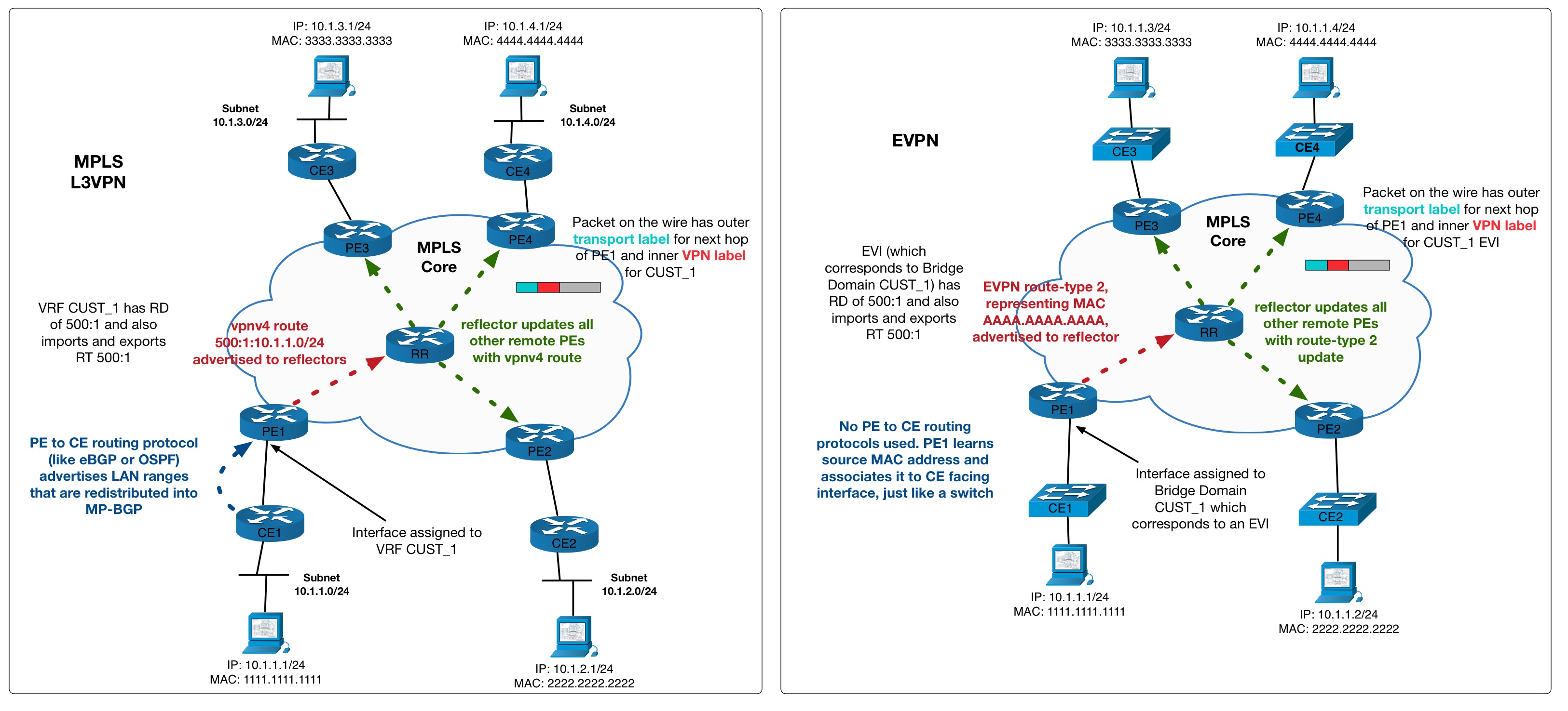
In EVPN, customer devices tend to be switches rather than routers. PE-CE routing protocols, like eBGP, aren’t used since it operates over layer 2. The Service Provider appears as one big switch. In this sense, it accomplishes the same as VPLS but (among other differences) uses BGP to distribute MAC address information, rather than using a full mesh of pseudowires.
EVPN uses an EVI, or Ethernet Virtual Identifier, to identify a specific instance of EVPN as it maps to a bridge domain. For the purposes of this overview, you can think of an EVI as being quasi-equivalent to a VRF. A customer facing interface will be put into a bridge domain (layer 2 broadcast domain), which will have an EVI identifier associated with it.
The MAC address learning that EVPN utilizes what is called control-plane learning, since it is BGP (a control-plane routing protocol) that distributes the MAC address information. This is in contrast to data-plane learning, which is how a standard switch learns MAC addresses – by associating the source MAC address of a frame to the receiving interface.
The following Cisco IOS-XR config shows an EVPN bridge domain and edge interface setup, side by side with a MPLS L3VPN setup for comparison:
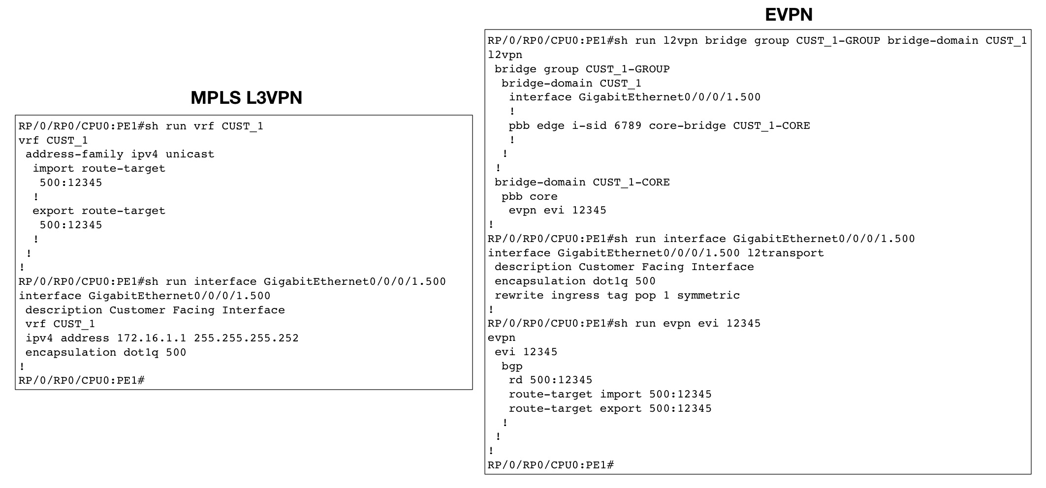
NB. For MPLS L3VPN config the RD config (which is usually configured under CE-PE eBGP config) is not shown. PBB config is shown in the EVPN Bridge domain, this will be explained further into the blog.
EVPN seems simple enough at first glance, but it has a scaling problem, which PBB can ultimately help with…
Any given customer site can have hundreds or even thousands of MAC addresses, as opposed to just one subnet (as in an MPLS L3VPN environment). The number of updates and withdrawals that BGP would have to send could be overwhelming if it needed to make adjustments for MAC addresses appearing and disappearing – not to mention the memory requirements. And you can’t summarise MAC addresses like you can IP ranges. It would be like an MPLS L3VPN environment advertising /32 prefixes for every host rather than just one prefix for the subnet. We need a way to summarise or aggregate the MAC addresses.
Here’s where PBB comes in…
PBB – Provider Backbone Bridging (802.1ah)
PBB can help solve the EVPN scaling issue by performing one key function – it maps each customer MAC address to the MAC address of the attaching PE. Customer MAC addresses are called C-MACs. The PE MAC addresses are call B-MACs (or Bridge MACs).
This works by adding an extra layer 2 header to frame as it is forwarded from one site to another across the provider core. The outer layer 2 header has a destination B-MAC address of the PE device that the inner frames destination C-MAC is associated with. As a result, PBB is often called MAC-in-MAC. This diagram illustrates the concept:

NB. In PBB terminology the provider devices are called Bridges. So a BEB (Backbone Edge Bridge) is a PE and a BCB (Backbone Core Bridge) is a P. For sake of simplicity, I will continue to use PE/P terminology. Also worth noting is that PBB diagrams often show service provider devices as switches, to illustrate the layer 2 nature of the technology – which I’ve done above.
In the above diagram the SID (or Service ID) represents a layer 2 broadcast domain similar to what an EVI represents in EVPN.
Frames arriving on a PE interface will be inspected and, based on certain characteristics, it will be mapped or assigned to a particular Service ID (SID).
The characteristics that determine what SID a frame belongs to can be a number of things:
- The customer assigned VLAN
- The Service Provider assigned VLAN
- Existing SID identifiers
- The interface it arrives on
- A combination of the above or other factors
To draw an analogy to MPLS L3VPN – the VRF that an incoming packet is assigned to is determined by whatever VRF is configured on the receiving interface (using ip vrf forwarding CUST_1 in Cisco IOS interface CLI).
Once the SID has been allocated, the entire frame is then encapsulated in the outer layer 2 header with destination MAC of the egress PE.
In this way C-MACs are mapped to either B-MACs or local attachment circuits. Most importantly however the core P routers do not need to learn all of the MAC addresses of the customers. They only deal with the MAC addresses of the PEs. This allows a PE to aggregate all of the attached C-MACs for a given customer behind its own B-MAC.
But how does a remote PE learn which C-MAC maps to which B-MAC?
In PBB learning is done in the data-plane, much like a regular layer 2 switch. When a PE receives a frame from the PBB core, it will strip off the outer layer 2 header and make a note of the source B-MAC (the ingress PE). It will map this source B-MAC to the source C-MAC found on the inner layer 2 header. When a frame arrives on a local attachment circuit, the PE will map the source C-MAC to the attachment circuit in the usual way.
PBB must deal with BUM traffic too. BUM traffic is Broadcast, Unknown Unicast or Multicast traffic. An example of BUM traffic is the arrival or frame for which the destination MAC address is unknown. Rather than broadcast like a regular layer 2 switch would, a PPB PE will set the destination MAC address of the outer layer 2 header to a special multicast MAC address that is built based on the SID and includes all the egress PEs that are part of the same bridge domain. EVPN uses a different method or handling BUM traffic but I will go into that later in the blog.
Overall, PBB is more complicated than the explanation given here, but this is the general principle (if you’re interested, see this doc that details how PBB can be combined with 802.1ad to add an aggregation layer to a provider network).
Now that we have the MAC-in-MAC features of PBB at our disposal, we can use it to solve the EVPN scaling problem and combine the two…
PBB-EVPN
With the help of PBB, EVPN can be adapted so that it deals with only the B-MACs.
To accomplish this, each EVPN EVI is linked to two bridge domains. One bridge domain is dedicated to customer MAC addresses and connected to the local attachment circuits. The other is dedicated to the PE routers B-MAC addresses. Both of these bridge domains are combined under the same bridge group.
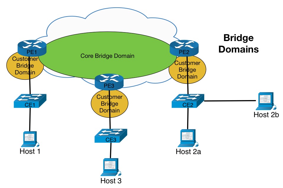
The PE devices will uses data-plane learning to build a MAC database, mapping each C-MAC to either an attachment circuit or the B-MAC of an egress PE. Source C-MAC addresses are learned and associated as traffic flows through the network just like PBB does.
The overall setup would look like this:

The only thing EVPN needs to concern itself with is advertising the B-MACs of the PE devices. EVPN uses control-plane learning and includes the B-MACs in the MP-BGP l2vpn evpn updates. For example, if you were to look at MAC address known to a particular EVI on a route-reflector, you would only see MAC address for PE routers.
Looking again at the configuration output that we saw above, we can get a better idea of how PBB-EVPN works:
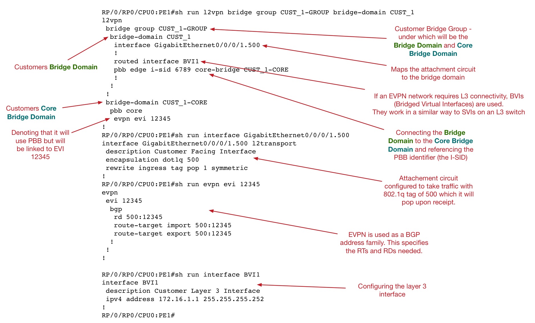
NB. I have added the concept of a BVI, or Bridged Virtual Interface, to the above output. This can be used to provide a layer 3 breakout or gateway similar to how an SVI works on a L3 switch.
You can view the MAC addresses information using the following command:
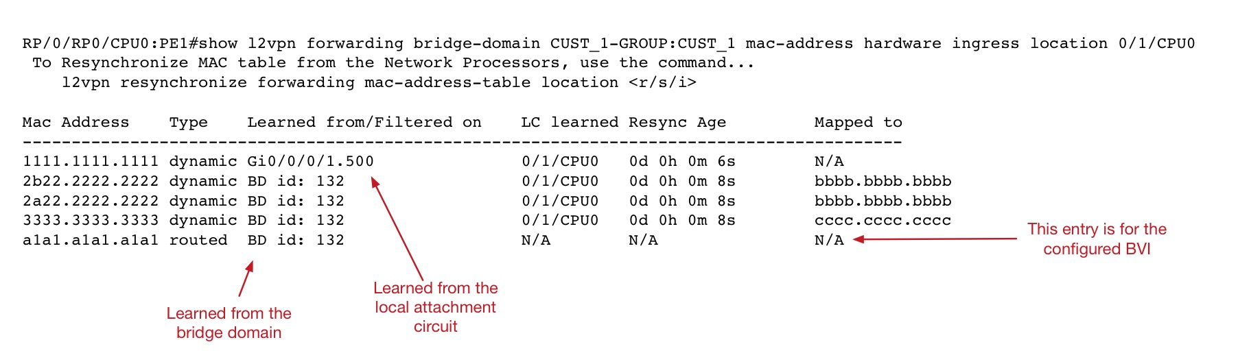
Now lets look at how PBB-EVPN handles BUM traffic. Unlike PBB on its own, which just sends to a multicast MAC address, PBB-EVPN will use unicast replication and send copies of the frame to all of the remote PEs that are in the same EVI. This is an EVPN method and the PE knows which remote PEs belong to the same EVI by looking in what is called a flood list.
But how does it build this flood list? To learn that, we need to look at EVPN route-types…
MPLS L3VPN sends VPNv4 routes in its updates. But EVPN send more than one “type” of update. The type of update, or route-type as it is called, will denote what kind of information is carried in the update. The route-type is part of the EVPN NLRI.
For the purposes of this blog we will only look at two route-types.
- Route-Type 2s, which carry MAC addresses (analogous to VPNv4 updates)
- Route-Type 3s, which carry information on the egress PEs that belong to an EVI.
It is these Route-Type 3s (or RT-3s for short) that are used to build the flood list.
When BUM traffic is received by a PE, it will send copies of the frame to all of its attachment circuits (except the one it received the frame on) and all of the PEs for which it has received a Route-Type 3 update. In other words, it will send to everything in its flood-list.
So the overall process for a BUM packet being forwarded across a PBB-EVPN backbone will look as follows:
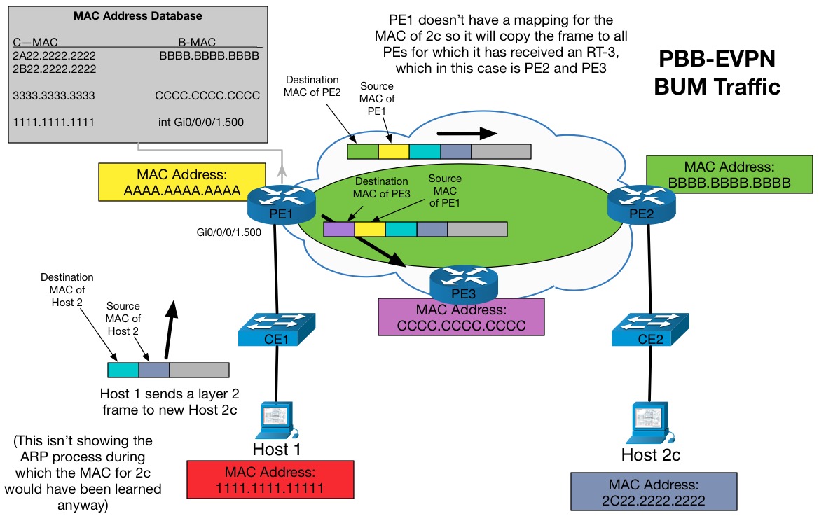
So that’s it, in a nutshell. In this way PBB and EVPN can work together to create an L2VPN network across a Service Provider.
There are other aspects of both PBB and EVPN, such as EVPN multi-homing using Ethernet Segment Identifiers or PBB MAC clearing with MIRP to name just a couple, but the purpose of this blog was to provide an introductory overview – specifically for those used to dealing with MPLS L3VPN. Thoughts are welcome, and as always, thank you for reading.

You must be logged in to post a comment.