netquirks
Exploring the quirks of Network Engineering
It’s not easy building GRE
The importance of having backup paths in a network isn’t a revelation to anyone. From HSRP on a humble pair of Cisco 887s to TI-LFA integration on an ASR9k, having a reliable backup path is a staple for all modern networks.
This quirk looks at the need for a backup path on a grand scale. We’ll look at a hypothetical scenario of a multi-national ISP losing a backup path to a whole region and how, as a rapid response solution, it builds a redundant path over a Transit Provider…
Scenario
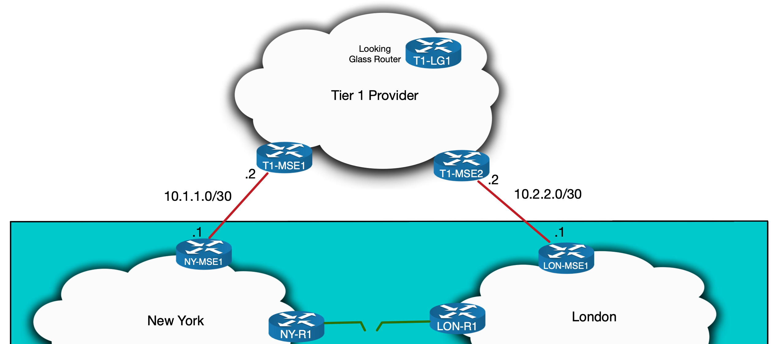
So here is our hypothetical Tier 2 Service Provider network. It is spread across three cities in three different countries and has various Peering and Transit connections throughout:

IS-IS and LDP is run internally. This includes the international links, resulting in one contiguous IGP domain. What’s important to note here is that New York only has a single link to the other countries and only has one Tier 1 Transit Provider.
The quirk
To setup this quirk, we need a link failure to take place. Let’s say a deep-sea dredger rips up the cable in the Atlantic going from New York to London.

New York doesn’t lose access – it still has a link to the rest of the network via Paris. However that link to Paris is now its sole connection to the rest of the network. In other words, New York no longer has that all important backup path. The situation is exacerbated when you learn that a repair boat won’t be sent to fix the undersea cable for weeks!
So what do you do?
You could invest in more fibre and undersea cabling to connect your infrastructure – arguably you should’ve already done this! But placing an order for a Layer 2 Service or contacting a Tier 1 Provider to setup CsC takes time. By all means, place the order. But in the meantime, you’ll need to set something up quickly in case New York to Paris fails and New York becomes completely isolated.
One option, and indeed the one we’ll explore in this blog, is to reconnect New York to London through your transit provider without waiting for an order or even involving them at all…
I should preface this by stating that this solution is neither scalable nor sustainable. But it is most definitely an interesting and … well… quirky work around that can be deployed at a pinch.
With that said, how do we actually do this?
In order to connect New York to London over another network, we’ll need to implement tunnelling of some kind. Specifically, we’ll look at creating a GRE tunnel between the MSEs in New York and London using the Tier 1 Transit Provider as the underlay network.
To put it in diagram form, our goal is to have something like this:

To guide us through this setup, I’ll tackle the process step by step using the following sections:
- Tunnel-end point Reachability
- Control Plane: The IPs of endpoints of the GRE tunnel will need reachability over the Tier 1 Transit Provider.
- Data Plane: Traffic between the endpoint must be able to flow. This section will examine what packet filtering might need adjusting.
- GRE tunnel configuration
- Control Plane: This covers the configuration and signalling of the GRE tunnel
- Data Plane: We’ll need to look at MTU and account for the additional overhead added by the GRE headers.
- Tunnel overlay protocols: Making sure IS-IS and LDP can be run over the GRE tunnel, including the proper transport addresses and metrics.
- Link Capacity: This new tunnel will need to be able to take the same amount of traffic that typically flows to and from New York. Given that our control over this is limited, we’ll assume that there is sufficient bandwidth on these links.
- RTBH: Any Remote Trigger Black Holing mechanisms that have been applied to your Transit ports may need to have exceptions made so it does not mistake your own traffic for a DDoS attack.
- Security: You could optionally encrypt the traffic transiting the Transit Providers network.
The goal of this quirk is to explore the routing and reachability side of the scenario so I will discuss the first 3 of the above points in detail and assume that link capacity, RTBH and security are already accounted for.
Downloadable Lab
This quirk considers the point of view of a large Service Provider with potentially hundreds of routers. However in order to demonstrate the configuration specifics and allow you to try the setup, I’ve built a small scale lab to emulate the solution. I’ve altered some of the output shown in this blog to make it appear more realistic. As such, the lab and output shown in this post don’t match each other verbatim. But I’ll turn to the lab towards the end in order to do a couple of traceroutes and for the most part the IP addressing and configuration match enough for you to follow along.
I built the lab in EVE-NG so it can be download as a zipped UNL file. I’ve also provided a zip file containing the configuration for each node, in case you’re using a different lab emulation program.

With that said, let’s take a look at how we’d set this up…
Tunnel-end point Reachability – Control Plane
We’ll start by putting some IP addressing on the topology:
(the addressing used throughout will be private, but in a real world scenario it would be public)
Now we might first try to build the tunnel directly between our routers, using 10.1.1.1 and 10.2.2.1 as the respective endpoints. But if we try to ping and trace from one to the other we see it fails:
RP/0/RSP0/CPU0:NY-MSE1#show route ipv4 10.2.2.1
Routing entry for 10.2.0.0/16
  Known via "bgp 500", distance 20, metric 0
  Tag 100, type external
  Installed Jul 12 15:36:41.110 for 2w2d
  Routing Descriptor Blocks
    10.1.1.2, from 10.1.1.2, BGP external
      Route metric is 0
  No advertising protos.
RP/0/RSP0/CPU0:NY-MSE1#ping 10.2.2.1
Wed Jul 26 15:26:21.374 EST
Type escape sequence to abort.
Sending 5, 100-byte ICMP Echos to 10.2.2.1, timeout is 2 seconds:
.....
Success rate is 0 percent (0/5)
RP/0/RSP0/CPU0:NY-MSE1#traceroute 10.2.2.1

Type escape sequence to abort.
Tracing the route to 10.2.2.1

 1  10.1.1.2 2 msec  1 msec  1 msec
 2  10.117.23.3 [MPLS: Label 43567 Exp 0] 34 msec  35 msec  35 msec
 3  10.117.23.17 [MPLS: Label 34234 Exp 0] 35 msec  36 msec  35 msec
 4  10.117.23.57 [MPLS: Label 94571 Exp 0] 36 msec  46 msec  35 msec
 5  10.117.23.23 [MPLS: Label 64066 Exp 0] 35 msec  35 msec  35 msec
 6   *  *  *
 7   *  *  *
 8   *  *  *
 9   *  *  *
RP/0/RSP0/CPU0:NY-MSE1#
From the traceroute we can see that traffic is entering an LSP in the Tier 1 MPLS core. The IPs we see are likely the loopback addresses of the P routers along the path. In spite of this limited visibility we can see the traffic isn’t reaching its destination – it is stopping at 10.117.23.23. But why?
Well, we don’t have full visibility of the Tier 1 Provider’s network, but they are likely restricting access to the transport subnets used to connect to their downstream customers. This is a common practice and is designed to, among other things, prevent customers from having access to networks that their Tier 1 edge devices exist on. Traffic should never go to these transport addresses, they should only go through them.
This means that when we see the traceroute stop at 10.117.23.23, this may very well be an ACL or filter on T1-MSE2 blocking traffic to 10.2.2.0/30 from an unauthorised source.

As a result of this, we’ll have to advertise a subnet to the Tier1 Provider from each side and have them act as the tunnel endpoints. Tier1 Providers typically don’t accept any prefix advertisement smaller than a /24 so in this case we’ll have no choice but to sacrifice two such ranges – one for each site. See why I mentioned this is not scalable?
Before we allocate these ranges, I’m going to assume the following points have already been fulfilled:
- The /24 address ranges are available and unused: let’s say we have a well documented IPAM (IP Address Management) system and can find a couple of /24s.
- The Transit Provider will accept the prefixes we advertise – meaning our RIR records are up to date and any RPKI ROAs are correctly configured so that the Transit Provider will not have any problems accepting the /24s advertised over BGP.
With these assumptions in place, we’ll start by allocating a subnet for each site (again, pretend these are public):
- New York subnet: 172.16.10.0/24
- London subnet: 172.16.20.0/24
At this point we need to see what the Transit Provider sees in order to make sure our routes are being received correctly. For this we’ll use a Looking Glass. To illustrate this, I’ve invented a hypothetical Transit Provider called TEAR1 Limited (a bad pun I know, but fit for our purposes 😛 ). I’ve put together images demonstrating what a Looking Glass website for TEAR1 might look like. First, we’ll specify that we want to find BGP routing information about 172.16.10.0:

After clicking submit, we might get a response similar to what you see below:

So what can we make out from the above output…? We can see, for example, that T1-LG1 is receiving the prefix from what looks like a Route Reflector (evident by the existence of a Cluster List in the BGP output) and from what is probably the T1-MSE1 Edge Router that receives the prefix from our ISP. The path to the Edge Router is being preferred, since it has a Cluster List length of zero. T1-LG1 could itself be a Reflector within TEAR1. It’s difficult to tell much more without knowing the full internal topology of TEAR1, but the main take home here is that is it sees a /16, rather than the more specific /24s. This is fine at this point – we haven’t configured anything yet. And indeed if we check NY-MSE1 we can see that we are originating a /16 as part of our normal prefix advertisements to Transit Providers:
RP/0/RSP0/CPU0:NY-MSE1#show route ipv4 172.16.0.0/16

Routing entry for 172.16.0.0/16
  Known via "static", distance 1, metric 0 (connected)
  Installed May 26 12:53:27.539 for 8w1d
  Routing Descriptor Blocks
    directly connected, via Null0
      Route metric is 0, Wt is 1
  No advertising protos.
RP/0/RSP0/CPU0:NY-MSE1#sh bgp ipv4 uni neigh 10.1.1.2 adv | in 172.16.0.0
172.16.0.0/16     10.1.1.1   Local           500i
RP/0/RSP0/CPU0:NY-MSE1#
Here we’re using a null route for the subnet. This is common within Service Providers. The null route is redistributed into BGP and advertised to TEAR1. This isn’t a problem since within our Service Provider there will be plenty of subnets with the 172.16.0.0/16 supernet – meaning there will always be more specific routes to follow. We could have alternatively used BGP aggregation.
Regardless of how this is done, we need to configure NY-MSE1 to advertise 172.16.10.0/24 to TEAR1 and LON-MSE1 to advertise 172.16.20.0/24. We could use static null routes here too, but remember the goal is to have these IPs be the endpoints of the GRE tunnel. With this in mind, we’ll use loopbacks and advertise them into BGP using the network statement. The overall configuration is as follows:
! (NY-MSE1)
interface Loopback10
 description Temporary GRE end-point
 ipv4 address 172.16.10.1 255.255.255.0
!
router bgp 500
 address-family ipv4 unicast
  network 172.16.10.0/24
(I’ve only shown the config for the New York side but the London side is analogous – obviously replacing 172.16.10.0 with 172.16.20.0. To save showing duplicate output, I will sometimes only show the New York side, but know that in those cases, the equivalent substituted config is on the London side.)
To advertise these ranges to TEAR1 we’ll need to adjust our outbound BGP policies.
I’ll pause here to note that filtering on both the control plane and data planes at a Service Provider edge is a complex subject. The CLI I’ve shown here is grossly oversimplified just to demonstrate the parts relevant to this quirk (including a couple of hypothetical communities that could be used for various routing policies). The ACL and route policies in a real network will be more complicated and cover more aspects of routing security, including anti-spoofing and BGP hi-jack prevention. That being said, here is the config we need to apply:
! (NY-MSE1)
router bgp 500
  address-family ipv4 unicast
   network 172.16.10.0/24
  !
 neighbor 10.1.1.2
  remote-as 100
  description TEAR1-BGP-PEER
  address-family ipv4 unicast
   send-community-ebgp
   route-policy TEAR1-OUT in
   route-policy TEAR1-IN in
   remove-private-AS
  !
!
route-policy TEAR1-OUT
  if community matches-any NO-TRANSIT then
    drop
  elseif community matches-any NEW-YORK-ORIGIN and destination in OUR-PREFIXES then
    pass
  elseif destination in (172.16.10.0/24) then
    set community (no-export)
    pass
  else
    drop
  endif
end-policy
And indeed if we soft clear the BGP sessions and check the Looking Glass again, we can see that TEAR1 now sees both /24 subnets.
RP/0/RSP0/CPU0:NY-MSE1#clear bgp ipv4 unicast 10.1.1.2 soft
RP/0/RSP0/CPU0:NY-MSE1#sh bgp ipv4 uni neigh 10.1.1.2 adv | include 172.16.10.0
172.16.10.0/24     10.1.1.1   Local           500i
RP/0/RSP0/CPU0:NY-MSE1#

RP/0/RSP0/CPU0:LON-MSE1#clear bgp ipv4 unicast 10.2.2.2 soft
RP/0/RSP0/CPU0:LON-MSE1#sh bgp ipv4 uni neigh 10.2.2.2 adv | include 172.16.20.0
172.16.20.0/24     10.2.2.1   Local           500i
RP/0/RSP0/CPU0:LON-MSE1#
You might’ve noticed in the above output the inclusion of the no-export community. This is done to make sure that TEAR1 does not advertise these /24s to any of its fellow Tier 1 Providers and pollute the internet further. By “polluting the internet” I mean introducing unnecessary prefixes into the global internet routing table. In this case, we are adding two /24s which, from the point of view of the rest of the internet, aren’t needed since we’re already advertising the /16. We can’t make TEAR1 honour the no-export community, but it is a reasonable precaution to put in place nonetheless.
This covers control plane advertisements to TEAR1. But we also need to think about how LON-MSE1 sees NY-MSE1s loopback and vice versa. Each MSE should see the GRE tunnel endpoint of the other over the TEAR1 connection. Depending on how we perform redistribution, we might see these tunnel endpoints in iBGP or in our IGP. But we don’t want them to see each over our own core or else that is the path the tunnel will take!
In addition to this, we don’t want TEAR1 to advertise our own IP addresses back to us. Most ISPs filter against this anyways, and even if we didn’t, BGP loop-prevention (seeing our own ASN in the AS_PATH attribute) would prevent our MSEs from accepting them.
The cleanest way to ensure NY-MSE1 has a best path for 172.16.20.0 via TEAR1 (and vice versa) is a static route:
! NY-MSE1
router static
 address-family ipv4 unicast
  172.16.20.1/32 TenGigE0/0/0/1 10.1.1.2 description GRE_Tunnel

! LON-MSE1
router static
 address-family ipv4 unicast
  172.16.10.1/32 TenGigE0/0/0/1 10.2.2.2 description GRE_Tunnel

RP/0/RSP0/CPU0:NY-MSE1#sh ip ro 172.16.20.1

Routing entry for 172.16.20.1/32
  Known via "static", distance 1, metric 0
  Installed Jul 7 18:34:18.727 for 1w2d
  Routing Descriptor Blocks
    10.1.1.2, via TenGigE0/0/0/1
      Route metric is 0, Wt is 1
  No advertising protos.
RP/0/RSP0/CPU0:NY-MSE1#
This will make sure that the tunnel is built over the Transit Provider. The data plane needs to be adjusted next, to allow the actual traffic to flow…
Tunnel-end point Reachability – Data Plane
Many Service Providers will apply inbound filters on Peering and Transit ports both on the control plane and data plane. This is done to, among other things, prevent IP spoofing. For example, any outbound traffic should have a source address that is part of the Service Providers address space (or from the PI Space of any of it customers). Similarly, any inbound traffic should have a source address that is not part of their customer address space. These are the types of things we’ll need to consider when opening up the data plane for our GRE tunnel.
For this scenario, let’s assume we block inbound traffic that is sourced from our own address space. This would prevent spoofed traffic crossing our network, but it would also block traffic from one of our GRE tunnel endpoints to the other. We’ll need to adjust the inbound ACL and to make this as secure as possible we should only allowing GRE traffic from and to the relevant /32 endpoints.
I’ve omitted the full details of this ACL, since in real life it would be too long to show. However here is the addition we’d need to make (assuming no reject statements before index 10):
! NY-MSE1
interface TenGigE0/0/0/1
 description Link to T1-MSE1
 ipv4 address 10.1.1.1 255.255.255.252
 ipv4 access-group FROM-TRANSIT ingress
!
ipv4 access-list IN-FROM-TRANSIT
 <<output omitted>>
 10 permit gre host 172.16.20.1 host 172.16.10.1
 <<output omitted>>
!
We’re now in a position to test connectivity – remembering to source from loopback10 so that LON-MSE1 has a return route:
RP/0/RSP0/CPU0:NY-MSE1#traceroute 10.2.2.1 source loopback 10

Type escape sequence to abort.
Tracing the route to 172.16.20.1

 1  10.1.1.2 2 msec  1 msec  1 msec
 2  10.117.23.3 [MPLS: Label 43567 Exp 0] 34 msec  35 msec  35 msec
 3  10.117.23.17 [MPLS: Label 34234 Exp 0] 35 msec  36 msec  35 msec
 4  10.117.23.57 [MPLS: Label 94571 Exp 0] 36 msec  46 msec  35 msec
 5  10.117.23.23 [MPLS: Label 64066 Exp 0] 35 msec  35 msec  35 msec
 6  10.2.2.1 msec *  60 msec
RP/0/RSP0/CPU0:NY-MSE1#
Success, it works! We have loopback to loopback reachability across TEAR1 and we didn’t even need to give them so much as a phone call. To put this in diagram format, here is where we are at:

We’re now ready to configure the GRE tunnel.
Configuring the Tunnel – Control Plane
The GRE configuration itself is fairly straight forward. We’ll configure the tunnel endpoint on each router, specifying the loopbacks as the sources. We also need to allocate IPs on the tunnel interfaces themselves. These will form an internal point-to-point subnet that will be used to establish the IS-IS and LDP neighborships we need. Let’s allocate 192.168.1.0/30, with NY-MSE1 being .1 and LON-MSE1 being .2.
The config looks like this:
! NY-MSE1
interface tunnel-ip100
 ipv4 address 192.168.1.1/30
 tunnel mode gre ipv4
 tunnel source Loopback10
 tunnel destination 172.16.20.1
!

! LON-MSE1
interface tunnel-ip100
 ipv4 address 192.168.1.2/30
 tunnel mode gre ipv4
 tunnel source Loopback10
 tunnel destination 172.16.10.1
!
Checking the GRE tunnel shows that it is up:
RP/0/RSP0/CPU0:NY-MSE1#sh interface tunnel-ip 100 detail
tunnel-ip100 is up, line protocol is up
  Interface state transitions: 3
  Hardware is Tunnel
  Internet address is 192.168.1.1/30
  MTU 1500 bytes, BW 100 Kbit (Max: 100 Kbit)
     reliability 255/255, txload 2/255, rxload 2/255
  Encapsulation TUNNEL_IP,  loopback not set,
  Last link flapped 1w2d
  Tunnel TOS 0
  Tunnel mode GRE IPV4
  Keepalive is disabled.
  Tunnel source 172.16.10.1(Loopback100), destination 172.16.20.1/32
  Tunnel TTL 255
  Last input 00:00:00, output 00:00:00
  Last clearing of "show interface" counters never
  5 minute input rate 1000 bits/sec, 1 packets/sec
  5 minute output rate 1000 bits/sec, 1 packets/sec
     264128771 packets input, 58048460659 bytes, 34 total input drops
     0 drops for unrecognized upper-level protocol
     Received 0 broadcast packets, 0 multicast packet
     115204515 packets output, 72846125759 bytes, 0 total output drops
     Output 0 broadcast packets, 0 multicast packets
RP/0/RSP0/CPU0:NY-MSE1#sh interface tunnel-ip 100 brief

               Intf       Intf        LineP              Encap  MTU        BW
               Name       State       State               Type (byte)    (Kbps)
--------------------------------------------------------------------------------
              ti100          up          up          TUNNEL_IP  1500        100


RP/0/RSP0/CPU0:LON-MSE1#sh interfaces tunnel-ip100 detail
tunnel-ip100 is up, line protocol is up
  Interface state transitions: 5
  Hardware is Tunnel
  Internet address is 192.168.1.2/30
  MTU 1500 bytes, BW 100 Kbit (Max: 100 Kbit)
     reliability 255/255, txload 2/255, rxload 2/255
  Encapsulation TUNNEL_IP,  loopback not set,
  Last link flapped 1w2d
  Tunnel TOS 0
  Tunnel mode GRE IPV4
  Keepalive is disabled.
  Tunnel source 172.16.20.1 (Loopback100), destination 172.16.10.1/32
  Tunnel TTL 255
  Last input 00:00:00, output 00:00:00
  Last clearing of "show interface" counters never
  5 minute input rate 1000 bits/sec, 1 packets/sec
  5 minute output rate 1000 bits/sec, 1 packets/sec
     115176196 packets input, 73259625130 bytes, 0 total input drops
     0 drops for unrecognized upper-level protocol
     Received 0 broadcast packets, 0 multicast packets
     264158130 packets output, 57031343960 bytes, 0 total output drops
     Output 0 broadcast packets, 0 multicast packets
RP/0/RSP0/CPU0:LON-MSE1#
So now we have the GRE tunnel up and running. Before we look at the MTU changes, I want to demonstrate how the MTU issue manifests itself by configuring the overlay protocols first…
Tunnel overlay protocols – LDP
The LDP configuration is, on the face of it, quite simple.
! Both LON-MSE1 and NY-MSE1
mpls ldp
 interface tunnel-ip100
  address-family ipv4
  !
 !
!
This will actually cause the session to come up, however on closer inspection the setup is not a typical one. (in this output NY-MSE and LON-MSE have loopback0 addresses of 2.2.2.2/32 and 22.22.22.22/32 respectively).
RP/0/0/CPU0:NY-MSE1#sh mpls ldp discovery
Thu Jul 23 19:52:06.959 UTC

Local LDP Identifier: 2.2.2.2:0
Discovery Sources:
  Interfaces:

    <<output to core router omitted>>

    tunnel-ip100 : xmit/recv
      VRF: 'default' (0x60000000)
      LDP Id: 22.22.22.22:0, Transport address: 22.22.22.22
          Hold time: 15 sec (local:15 sec, peer:15 sec)
          Established: Jul 23 19:50:14.967 (00:01:52 ago)

RP/0/0/CPU0:NY-MSE1#sh mpls ldp neighbor
Thu Jul 23 19:54:21.940 UTC

    <<output to core router omitted>>

Peer LDP Identifier: 22.22.22.22:0
  TCP connection: 22.22.22.22:54279 - 2.2.2.2:646
  Graceful Restart: No
  Session Holdtime: 180 sec
  State: Oper; Msgs sent/rcvd: 25/25; Downstream-Unsolicited
  Up time: 00:02:30
  LDP Discovery Sources:
    IPv4: (1)
      tunnel-ip100
    IPv6: (0)
  Addresses bound to this peer:
    IPv4: (5)
      10.2.2.1       10.20.24.2     22.22.22.22    172.16.20.1
      192.168.1.2
    IPv6: (0)

RP/0/0/CPU0:NY-MSE1#
To explain the above output it’s worth quickly reviewing LDP (see here for a cheat sheet). LDPs Hellos, with a TTL of 1 are sent to 224.0.0.2 (the all routers multicast address) out of all interfaces with LDP enabled. This includes the GRE tunnel. This means that LON-MSE1 and NY-MSE1 establish an Hello Adjacency over the tunnel. Once this Adjacency is up, the router with the lower LDP Router ID will establish a TCP Session to the transport address of the other (from its own transport address). The transport address is included in the LDP Hellos. This address defaults to the LDP Router ID which in turn defaults to the highest numbered loopback. This allocation of the Router ID only occurs once (on IOS-XR) when LDP is first initialised and from then on, only when the existing Router ID is changed. As a result, depending on the order in which loopbacks and LDP are introduced, the Router ID might not necessarily be the current highest loopback address. In the output above we can see that the TCP Session is established between the loopback0s of each router. This is the loopback used to identify the node and is used for things like the source address of iBGP sessions. What’s key here is that each routers path to the other routers loopback0 address is internal – over the IGP. This means the TCP Session is established over our own core.

This isn’t a problem initially – LDP would come up and labels would be exchanged. But if our last link to New York via Paris goes down, this will cause the TCP Session to drop. It should come back up with IS-IS configured over the GRE tunnel, but this kind of disruption, combined with delays associated with LDP-IGP synchronisation, could result in significant downtime.
The wiser option is to configure the transport addresses to the be the GRE tunnel endpoints. This will ensure the TCP Session will be established over the GRE tunnel from the start…
! NY-MSE1
mpls ldp
 address-family ipv4
 !
 interface tunnel-ip100
  address-family ipv4
   discovery transport-address 192.168.1.1
  !
 !
!

! LON-MSE1
mpls ldp
 address-family ipv4
 !
 interface tunnel-ip100
  address-family ipv4
   discovery transport-address 192.168.1.2
  !
 !
!
Once this is done we can see the transport address changes accordingly:
RP/0/0/CPU0:NY-MSE1#sh mpls ldp discovery
Fri Jul 24 23:30:40.832 UTC

Local LDP Identifier: 2.2.2.2:0
Discovery Sources:
  Interfaces:

    <<output to core router omitted>>

    tunnel-ip100 : xmit/recv
      VRF: 'default' (0x60000000)
      LDP Id: 22.22.22.22:0, Transport address: 192.168.1.2
          Hold time: 15 sec (local:15 sec, peer:15 sec)
          Established: Jul 24 23:29:58.135 (00:00:42 ago)

RP/0/0/CPU0:NY-MSE1#sh mpls ldp neighbor
Fri Jul 24 23:30:44.472 UTC

    <<output to core router omitted>>

Peer LDP Identifier: 22.22.22.22:0
  TCP connection: 192.168.1.2:43187 - 192.168.1.1:646
  Graceful Restart: No
  Session Holdtime: 180 sec
  State: Oper; Msgs sent/rcvd: 23/23; Downstream-Unsolicited
  Up time: 00:00:32
  LDP Discovery Sources:
    IPv4: (1)
      tunnel-ip100
    IPv6: (0)
  Addresses bound to this peer:
    IPv4: (5)
      10.2.2.1       10.20.24.2     22.22.22.22    172.16.20.1
      192.168.1.2
    IPv6: (0)

RP/0/0/CPU0:NY-MSE1#
It’s also a good idea to manually configure the LDP Router ID to ensure that transport address connectivity is not reliant on an automatic process (I found when labbing this scenario that the LDP Router ID was, at times, defaulting to loopback10 used for the GRE Tunnel. Since I was not redistributing this loopback into IS-IS, this resulted in the neighboring P router not having a route to this address to establish the TCP session. Hardcoding the LDP Router ID to loopback0s address solved this).
Now that IS-IS is up, we can move on to the IGP configuration.
Tunnel overlay protocols – IS-IS
The IS-IS configuration across the GRE tunnel is done just like any interface. The only thing to remember here is to set the metric to be high enough such that under normal circumstances traffic will go via Paris (output from here on is taken from the downloadable lab, in case you notice subtle differences from the output given so far).
RP/0/0/CPU0:NY-MSE1#conf t
Mon Jul 27 21:51:08.282 UTC
RP/0/0/CPU0:NY-MSE1(config)#router isis LAB
RP/0/0/CPU0:NY-MSE1(config-isis)# interface tunnel-ip100
RP/0/0/CPU0:NY-MSE1(config-isis-if)#  circuit-type level-2-only
RP/0/0/CPU0:NY-MSE1(config-isis-if)#  point-to-point
RP/0/0/CPU0:NY-MSE1(config-isis-if)#  address-family ipv4 unicast
RP/0/0/CPU0:NY-MSE1(config-isis-if-af)#   metric 1000
RP/0/0/CPU0:NY-MSE1(config-isis-if-af)#   mpls ldp sync
RP/0/0/CPU0:NY-MSE1(config-isis-if-af)#  !
RP/0/0/CPU0:NY-MSE1(config-isis-if-af)#commit
Mon Jul 27 21:51:18.292 UTC
RP/0/0/CPU0:Jul 27 21:51:18.541 : config[65742]: %MGBL-CONFIG-6-DB_COMMIT :
Configuration committed by user 'user1'. Use 'show configuration commit changes
1000000073' to view the changes.
RP/0/0/CPU0:NY-MSE1(config-isis-if-af)#RP/0/0/CPU0:Jul 27 21:51:28.231 :
isis[1010]: %ROUTING-ISIS-5-ADJCHANGE : Adjacency to LON-MSE1 (tunnel-ip100)
(L2) Up, New adjacency
RP/0/0/CPU0:Jul 27 21:51:28.751 : isis[1010]: %ROUTING-ISIS-4-SNPTOOBIG : L2 SNP
size 1492 too big for interface tunnel-ip100 MTU 1476, trimmed to interface MTU

RP/0/0/CPU0:NY-MSE1(config-isis-if-af)#
RP/0/0/CPU0:Jul 27 21:51:52.309 : config[65742]: %MGBL-SYS-5-CONFIG_I : Configured
from console by user1
RP/0/0/CPU0:NY-MSE1#show isis neighbor
Mon Jul 27 21:51:57.699 UTC

IS-IS LAB neighbors:
System Id      Interface        SNPA           State Holdtime Type IETF-NSF
P1             Gi0/0/0/2        *PtoP*         Up    24       L2   Capable
LON-MSE1       ti100            *PtoP*         Up    20       L2   Capable

Total neighbor count: 2
RP/0/0/CPU0:NY-MSE1#
Once IS-IS comes up, you might notice the following log message:
RP/0/0/CPU0:Jul 27 21:54:23.419 : isis[1010]: %ROUTING-ISIS-4-SNPTOOBIG : L2
SNP size 1492 too big for interface tunnel-ip100 MTU 1476, trimmed to interface MTU
This leads us to the last topic we need to explore, MTU…
MTU
To consider MTU, let’s first see what the MTU currently is:
RP/0/0/CPU0:NY-MSE1#show interface GigabitEthernet 0/0/0/1
Mon Jul 27 22:04:12.558 UTC
GigabitEthernet0/0/0/1 is up, line protocol is up
  Interface state transitions: 1
  Hardware is GigabitEthernet, address is 5000.000c.0002 (bia 5000.000c.0002)
  Internet address is 10.1.1.1/30
  MTU 1514 bytes, BW 1000000 Kbit (Max: 1000000 Kbit)
     reliability 255/255, txload 0/255, rxload 0/255
  Encapsulation ARPA,
  Full-duplex, 1000Mb/s, unknown, link type is force-up
  <<output omitted>>
In IOS-XR the 14 bytes of the Layer 2 header needs to be accounted for (6 bytes for Source MAC + 6 bytes for Destination MAC + 2 Bytes for the Ethertype) so the 1514 bytes in the above output equates to a Layer 3 MTU of 1500.
If we look at the GRE tunnel MTU it too shows 1500 and unlike the physical interface MTU it doesn’t need account for the layer 2 header.
RP/0/0/CPU0:NY-MSE1#show interface tunnel-ip100
Mon Jul 27 22:07:48.454 UTC
tunnel-ip100 is up, line protocol is up
  Interface state transitions: 1
  Hardware is Tunnel
  Internet address is 192.168.1.1/30
  MTU 1500 bytes, BW 100 Kbit (Max: 100 Kbit)
     reliability 255/255, txload 2/255, rxload 2/255
  Encapsulation TUNNEL_IP,  loopback not set,
  Last link flapped 1d00h
  Tunnel TOS 0
  Tunnel mode GRE IPV4,
  Keepalive is disabled.
  Tunnel source 172.16.10.1 (Loopback10), destination 172.16.20.1
  Tunnel TTL 255
  <<output omitted>>
But what the MTU in the above output doesn’t show is that the tunnel has to add a 24 byte GRE header, reducing the effective MTU of the link. If we use the following command we can see that the Layer 3 IPv4 MTU is 1476 (1500 -24):
RP/0/0/CPU0:NY-MSE1#show im database interface tunnel-ip100
Mon Jul 27 22:13:42.299 UTC

View: OWN - Owner, L3P - Local 3rd Party, G3P - Global 3rd Party, LDP - Local
      Data Plane
      GDP - Global Data Plane, RED - Redundancy, UL - UL

Node 0/0/CPU0 (0x0)

Interface tunnel-ip100, ifh 0x00000090 (up, 1500)
  Interface flags:          0x0000000000034457 (REPLICATED|STA_REP|TUNNEL
                            |IFINDEX|VIRTUAL|CONFIG|VIS|DATA|CONTROL)
  Encapsulation:            gre_ipip
  Interface type:           IFT_TUNNEL_GRE
  Control parent:           None
  Data parent:              None
  Views:                    UL|GDP|LDP|G3P|L3P|OWN

  Protocol        Caps (state, mtu)
  --------        -----------------
  None            gre_ipip (up, 1500)
  clns            clns (up, 1476)
  ipv4            ipv4 (up, 1476)
  mpls            mpls (up, 1476)

RP/0/0/CPU0:NY-MSE1#
This explains the IS-IS log message we were seeing:
RP/0/0/CPU0:Jul 27 21:54:23.419 : isis[1010]: %ROUTING-ISIS-4-SNPTOOBIG : L2
SNP size 1492 too big for interface tunnel-ip100 MTU 1476, trimmed to interface MTU
IS-IS is trying to send a packet that is bigger than 1476 bytes and so it must reduce the MTU size. This doesn’t have an impact on the IS-IS session in our case, but is worth noting.
To better understand the exact MTU breakdown, let’s visualise what happens when a packet arrives at NY-MSE1 headed for the GRE tunnel.
The packet arrives looking like this:
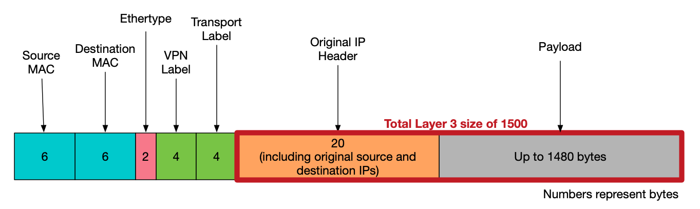
The MSE will then add the 24 bytes of GRE headers before sending it the Transit Provider, making the packet look like this:

So what is the impact of this? Will traffic be able to flow over the link?
Well in short, yes. But hosts will tend to sent packets of 1500 bytes (which includes the IP Header). With the additional Label and GRE headers in place, the packet will be fragmented as it is sent over TEAR1.
To illustrate this, I’ll turn to a pcap on EVE lab used to simulate this scenario. We’ll look at what happens if the link to Paris actual fails and our GRE tunnel is brought into action!
The lab contains a customer VRF with two sites, A and B. Loopback1 on the CE at each site is used to represent a LAN range. We can ping or trace from one site to another and watch its behaviour across the core. The lab includes a single link between the London and New York parts of the network used to represent the path via Paris. If we bring this link down, traffic will start to flow over the GRE tunnel. We can then do a pcap on NY-MSE1 to T1-MSE1 link to see the fragmentation. Here’s the setup:

First bring down our link to London:
P1(config)#int Gi4
P1(config-if)#shut
P1(config-if)#
*Jul 27 22:29:20.447: %LDP-5-NBRCHG: LDP Neighbor 44.44.44.44:0 (4) is DOWN
(Interface not operational)
*Jul 27 22:29:20.548: %CLNS-5-ADJCHANGE: ISIS: Adjacency to P2 (GigabitEthernet4)
Down, interface deleted(non-iih)
*Jul 27 22:29:20.549: %CLNS-5-ADJCHANGE: ISIS: Adjacency to P2 (GigabitEthernet4)
Down, interface deleted(non-iih)
P1(config-if)#
Then do a trace and ping while pcap’ing the outbound interface to T1-MSE1:
CE1#trace 192.168.70.1 source loopback1
Type escape sequence to abort.
Tracing the route to 192.168.70.1
VRF info: (vrf in name/id, vrf out name/id)
  1 172.30.1.9 46 msec 5 msec 1 msec
  2 10.10.14.4 [AS 500] [MPLS: Labels 1408/2107 Exp 0] 43 msec 15 msec 22 msec
  3 10.10.24.2 [AS 500] [MPLS: Labels 24003/2107 Exp 0] 46 msec 13 msec 12 msec
  4 192.168.1.2 [AS 500] [MPLS: Labels 24001/2107 Exp 0] 53 msec 15 msec 12 msec
  5 10.20.24.4 [AS 500] [MPLS: Labels 2402/2107 Exp 0] 31 msec 34 msec 13 msec
  6 172.30.1.13 [AS 500] [MPLS: Label 2107 Exp 0] 32 msec 13 msec 20 msec
  7 172.30.1.14 [AS 500] 54 msec *  44 msec
CE1#ping 192.168.70.1 source loopback 1 size 1500
Type escape sequence to abort.
Sending 5, 1500-byte ICMP Echos to 192.168.70.1, timeout is 2 seconds:
Packet sent with a source address of 192.168.60.1
!!!!!
Success rate is 100 percent (5/5), round-trip min/avg/max = 18/38/111 ms
CE1#
The PCAP shows fragmentation taking place on the ICMP packets:
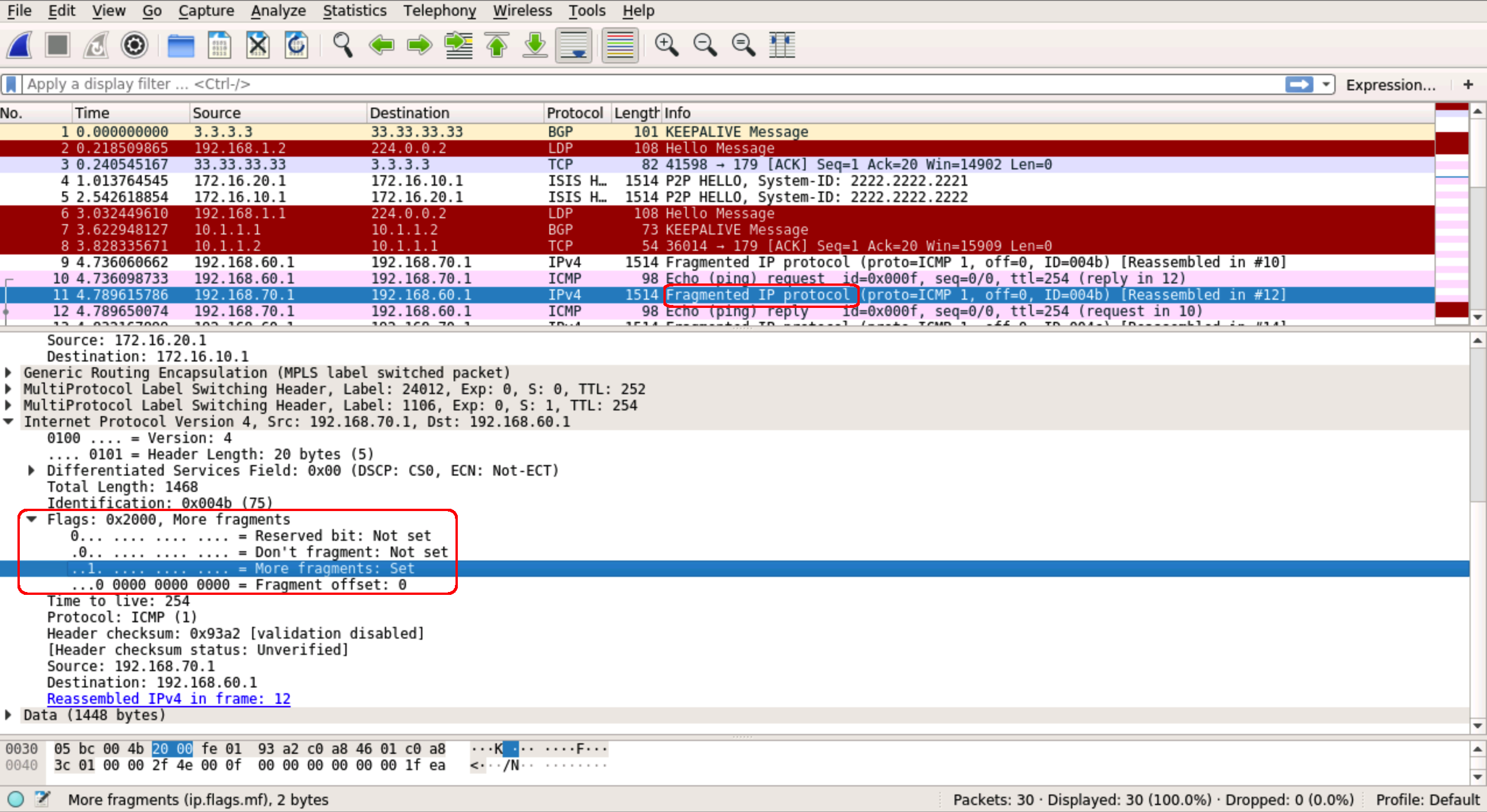
Indeed if we ping with the df bit set we see it doesn’t get through:
CE1#ping 192.168.70.1 source loopback1 size 1500 df-bit
Type escape sequence to abort.
Sending 5, 1500-byte ICMP Echos to 192.168.70.1, timeout is 2 seconds:
Packet sent with a source address of 192.168.60.1
Packet sent with the DF bit set
.....
Success rate is 0 percent (0/5)
CE1#
Fragmentation should generally be avoided where possible. To that end, we’ll need to adjust the MTU to allow our end host to sent at its usual 1500 bytes without fragmentation.
We will need to add 32 bytes to the already 1514 MTU. The breakdown is as follows:
- Original IP Header and Data – 1500
- VPN Label – 4
- Transport Label – 4
- GRE Header – 24
- Layer 2 Headers – 14
- TOTAL: 1546
So of we set the MTU to 1546 we’ll be able to send a packet of 1500 bytes across our core. Remember for the GRE tunnel we don’t need bother accounting for the 14 bytes of layer 2 overhead:
RP/0/0/CPU0:NY-MSE1(config)#interface tunnel-ip100
RP/0/0/CPU0:NY-MSE1(config-if)#mtu 1532
RP/0/0/CPU0:NY-MSE1(config-if)#interface GigabitEthernet0/0/0/1
RP/0/0/CPU0:NY-MSE1(config-if)#mtu 1546
RP/0/0/CPU0:NY-MSE1(config-if)#commit

RP/0/0/CPU0:LON-MSE1(config)#interface tunnel-ip100
RP/0/0/CPU0:LON-MSE1(config-if)#mtu 1532
RP/0/0/CPU0:LON-MSE1(config-if)#interface GigabitEthernet0/0/0/1
RP/0/0/CPU0:LON-MSE1(config-if)#mtu 1546
RP/0/0/CPU0:LON-MSE1(config-if)#commit
Once this done we can see that sending exactly 1500 bytes from our customer site works:
CE1#ping 192.168.70.1 source loopback1 size 1501 df-bit
Type escape sequence to abort.
Sending 5, 1501-byte ICMP Echos to 192.168.70.1, timeout is 2 seconds:
Packet sent with a source address of 192.168.60.1
Packet sent with the DF bit set
.....
Success rate is 0 percent (0/5)
CE1#ping 192.168.70.1 source loopback1 size 1500 df-bit
Type escape sequence to abort.
Sending 5, 1500-byte ICMP Echos to 192.168.70.1, timeout is 2 seconds:
Packet sent with a source address of 192.168.60.1
Packet sent with the DF bit set
!!!!!
Success rate is 100 percent (5/5), round-trip min/avg/max = 14/41/110 ms
CE1#
One final point to note here is that the Layer 3 MTU of the interface on the other end of the Transit link must be at least 1532 otherwise IS-IS will not come up across the GRE tunnel. This is unfortunately something that, as the Tier 2 Provider, we don’t control. In fact, any MTU along the part of the path that we don’t control could result in fragmentation. The best we can do in this case is to configure it and see. If IS-IS isn’t up after the MTU changes, we would have to revert and simply put up with the fragmentation.
So that’s it! An interesting solution to a somewhat rare and bespoke problem. Hopefully this blog has provided some insight into how Service Providers operate and how various technologies interrelate with one another to reach an end goal of maintaining redundancy. Again, I stress that this solution is not scalable, but I think it’s an entertaining look into what can be accomplished if you think outside the box. Feel free to download the lab and have a play around. Maybe you can see a different way to approach the scenario? Thoughts and feedback are welcome as always.

You must be logged in to post a comment.